Exploring the human genome with Bioconductor

Mission
Last time, we accessed data for the yeast genome and used several essential packages from the Bioconductor repository. In this post, I will load the BSgenome sequence object, genomic ranges and annotation data for the human genome and review some of the accessor functions for working with these data objects. Then I will use data from the cpgIslands package to generate visualization tracks using the Gviz package. To conclude, I will explore common strategies for accessing annotation data.
Let’s get started!
# Load packages
library(tidyverse)
theme_set(theme_light())
library(TxDb.Hsapiens.UCSC.hg19.knownGene)
library(Homo.sapiens) # Use with AnnotationDbi accessors e.g., columns(Homo.sapiens)
library(Biostrings)
library(GenomicRanges)
library(BSgenome.Hsapiens.UCSC.hg19)
library(AnnotationHub)
library(plyranges)
library(GenomicFeatures)
library(ggbio)
library(Gviz)
library(glue)
With the amazing TxDb package for the human genome (TxDb.Hsapiens.UCSC.hg19.knownGene), we can extract ranges for genes, transcripts, exons, promoters or other custom genomic ranges with minimal effort. We will use the genes() function to get the genomic ranges for all human genes.
human_txdb <- TxDb.Hsapiens.UCSC.hg19.knownGene # Genomic ragnes for genes

seqinfo(human_txdb)
## Seqinfo object with 93 sequences (1 circular) from hg19 genome:
## seqnames seqlengths isCircular genome
## chr1 249250621 <NA> hg19
## chr2 243199373 <NA> hg19
## chr3 198022430 <NA> hg19
## chr4 191154276 <NA> hg19
## chr5 180915260 <NA> hg19
## ... ... ... ...
## chrUn_gl000245 36651 <NA> hg19
## chrUn_gl000246 38154 <NA> hg19
## chrUn_gl000247 36422 <NA> hg19
## chrUn_gl000248 39786 <NA> hg19
## chrUn_gl000249 38502 <NA> hg19genes <- genes(human_txdb)Let’s do a quick visualization of the total gene count by chromosomes. To add a layer of information, I will use the glue package to combine chromosome name and gene count.
chrom_names <- c(paste0("chr", 1:22), 'chrX', 'chrY')

genes %>% as_tibble() %>%
  mutate(seqnames = as.character(seqnames)) %>%
  filter(seqnames %in% chrom_names) %>%
  group_by(seqnames) %>%
  count() %>%
  mutate(chrom_gene = glue('{seqnames} ({n})')) %>%
  ggplot(aes(n, fct_reorder(chrom_gene, n), fill = n)) +
  geom_col() +
  labs(title = "Gene count by chromosome",
       y = NULL,
       x = NULL) +
  theme(legend.position = 'none')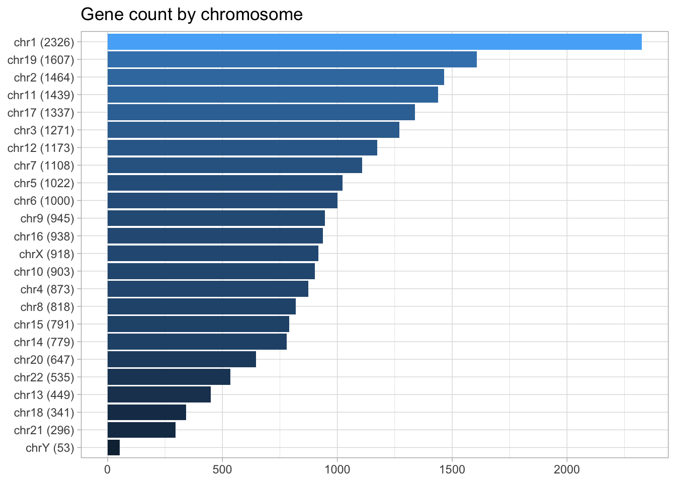
In the last example, I converted from GRanges to a data frame, filtered for standard chromosomes, tallied genes by chromosome and plotted the results with GGplot2. A simpler way to filter for standard chromosomes can be achieved with the function, keepStandardChromosomes(x) where x can be any Seqinfo object (TxDb).
CpG islands (CGIs)
CGIs are genomic regions with a higher frequency of CpG dinucleotide repeats. Many genes in vertebrate genomes have CGIs associated with their promoter regions. These CGIs are recognized as functionally important for regulating gene expression. CGIs with a lack of DNA methylation are associated with active promoter regions.
We will use the cpgIslands dataset to create an annotation data track and combine it with other tracks using the Gviz package. The tracks in the following plot include a representation of chromosome 7 with a red mark to specify the region of the CpG data, a ruler based on the min and max ranges of the CpG data, a track specifying the locations of CGIs and a final track for gene models in this region.
library(Gviz)
data(cpgIslands)
cpgIslands
## GRanges object with 10 ranges and 0 metadata columns:
## seqnames ranges strand
## <Rle> <IRanges> <Rle>
## [1] chr7 26549019-26550183 *
## [2] chr7 26564119-26564500 *
## [3] chr7 26585667-26586158 *
## [4] chr7 26591772-26593309 *
## [5] chr7 26594192-26594570 *
## [6] chr7 26623835-26624150 *
## [7] chr7 26659284-26660352 *
## [8] chr7 26721294-26721717 *
## [9] chr7 26821518-26823297 *
## [10] chr7 26991322-26991841 *
## -------
## seqinfo: 1 sequence from hg19 genome; no seqlengthsdata(geneModels)
# Data for hg19, chr7
gen <- genome(cpgIslands)
# Chromosome name
chr <- as.character(unique(seqnames(cpgIslands)))
# Ideogram track
itrack <- IdeogramTrack(genome = gen, chromosome = chr)
# Axis ruler track
gtrack <- GenomeAxisTrack()
# Add cpgIsland track
atrack <- AnnotationTrack(cpgIslands, name = "CpG")
# Add gene models track
grtrack <- GeneRegionTrack(geneModels, genome = gen,
chromosome = chr, name = "Gene Models")
#Annoation track for CPG island overlaps with promoters
promoters <- promoters(human_txdb, downstream = 100) %>%
filter(seqnames == "chr7")
subsetByOverlaps(cpgIslands, promoters, ignore.strand = TRUE)## GRanges object with 0 ranges and 0 metadata columns:
## seqnames ranges strand
## <Rle> <IRanges> <Rle>
## -------
## seqinfo: 1 sequence from hg19 genome; no seqlengths# Combine as list plot
plotTracks(list(itrack, gtrack, atrack, grtrack))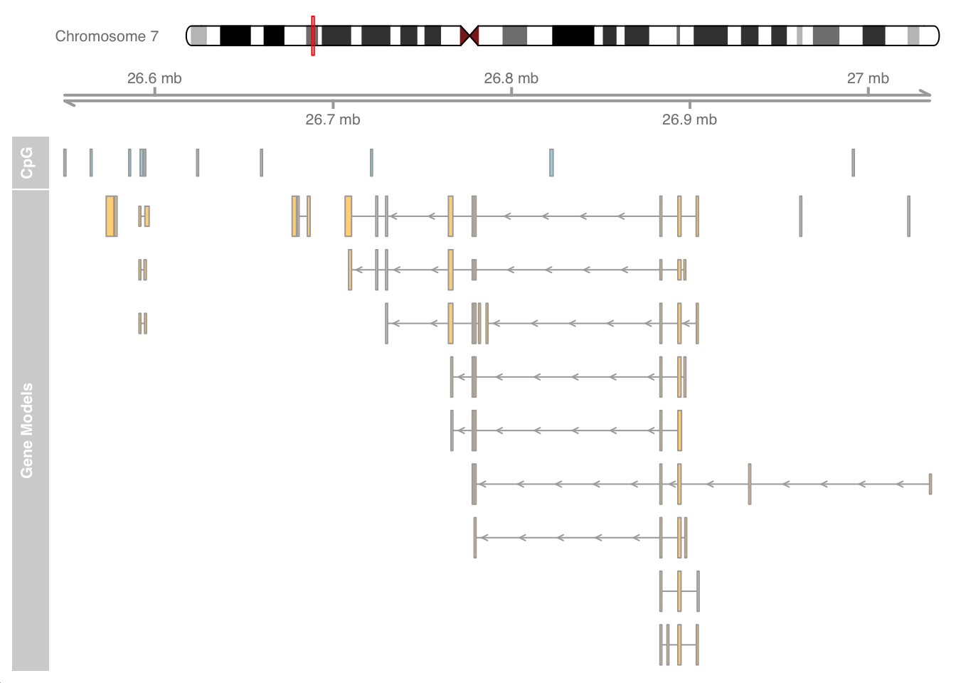
I borrowed the previous example from the Gviz vignette. Now that we are Gviz wizards, let’s create our own custom example using the gene info for the voltage sensing potassium (herg) channel in the human heart and surrounding regions on chromosome 2.
herg_channel <- GRanges("chr2:163227917-163695257", strand = "-")

# transcriptsBy(human_txdb, herg_channel) #to get sequences
genomeAxis <- GenomeAxisTrack(name="MyAxis")


anno_track <- AnnotationTrack(herg_channel, name = "Herg")

# Ideogram
ideoTrack <- IdeogramTrack(genome = "hg19", chromosome = "chr2")

hg19 <- c(chr2 = "hg19")
chrom = "chr2"

human_transcripts <- transcriptsBy(human_txdb, by = 'gene') %>%
  as_tibble() %>%
  filter(seqnames == "chr2")

geneTrack <- GeneRegionTrack(human_transcripts, genome = hg19,
                           chromosome = chrom, name = "Gene Models")

# Show chromosome band ID
plotTracks(list(ideoTrack, anno_track, geneTrack, genomeAxis),
           from = 162225917, to = 164697257)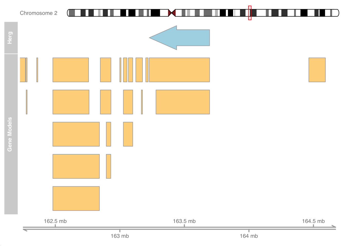
There are many more track possibilities with Gviz. We will revisit the package in a future post and show how we can utilize many different plot types.
Gene annotation
The default gene_id column for TxDb objects uses the NCBI Entrez ID nomenclature. Before, we get into the nitty-gritty of annotating genes, it’s worth noting that we may need to change our chromosome naming conventions to work with the annotation database of interest. The package, GenomeInfoDb makes this easy.
library(GenomeInfoDb)

chromNaming <- genomeStyles()
names(chromNaming) # See what organism genomes are available
## [1] "Arabidopsis_thaliana" "Caenorhabditis_elegans"
## [3] "Canis_familiaris" "Cyanidioschyzon_merolae"
## [5] "Drosophila_melanogaster" "Homo_sapiens"
## [7] "Mus_musculus" "Oryza_sativa"
## [9] "Populus_trichocarpa" "Rattus_norvegicus"
## [11] "Saccharomyces_cerevisiae" "Zea_mays"chromNaming$Homo_sapiens %>%
head() # See conventions for homosapiens## circular auto sex NCBI UCSC dbSNP Ensembl
## 1 FALSE TRUE FALSE 1 chr1 ch1 1
## 2 FALSE TRUE FALSE 2 chr2 ch2 2
## 3 FALSE TRUE FALSE 3 chr3 ch3 3
## 4 FALSE TRUE FALSE 4 chr4 ch4 4
## 5 FALSE TRUE FALSE 5 chr5 ch5 5
## 6 FALSE TRUE FALSE 6 chr6 ch6 6# E.g.
seqlevelsStyle(genes) <- "UCSC" # change chromosome naming conventions if desired
seqlevelsStyle(genes)## [1] "UCSC"Columns, keytypes and keys are the arguments that allow AnnotationDbi::select() to retrieve annotation data from the OrgDb database. In the following code chunk, I use columns() to see the available annotation and keytypes() to see the types of identifiers for the org.Hs.eg.db database object.
library(org.Hs.eg.db)
columns(org.Hs.eg.db) # available annotation resource databases for homo sapiens
## [1] "ACCNUM" "ALIAS" "ENSEMBL" "ENSEMBLPROT" "ENSEMBLTRANS"
## [6] "ENTREZID" "ENZYME" "EVIDENCE" "EVIDENCEALL" "GENENAME"
## [11] "GENETYPE" "GO" "GOALL" "IPI" "MAP"
## [16] "OMIM" "ONTOLOGY" "ONTOLOGYALL" "PATH" "PFAM"
## [21] "PMID" "PROSITE" "REFSEQ" "SYMBOL" "UCSCKG"
## [26] "UNIPROT"#keytypes(org.Hs.eg.db) # types of identifiers (often same as the columns() ouput)
#keys(org.Hs.eg.db) # returns keys (index) for the database contained in the OrgDb object
library(AnnotationDbi)
# Let's try an example using alpha-1-B glycoprotein (A1BG) as our gene of interest to annotate
AnnotationDbi::select(org.Hs.eg.db, keys = "A1BG", keytype = "SYMBOL",
columns = c("SYMBOL", "GENENAME", "CHR", "GO", "PROSITE"))## SYMBOL GENENAME CHR GO EVIDENCE ONTOLOGY PROSITE
## 1 A1BG alpha-1-B glycoprotein 19 GO:0002576 TAS BP PS50835
## 2 A1BG alpha-1-B glycoprotein 19 GO:0003674 ND MF PS50835
## 3 A1BG alpha-1-B glycoprotein 19 GO:0005576 HDA CC PS50835
## 4 A1BG alpha-1-B glycoprotein 19 GO:0005576 IDA CC PS50835
## 5 A1BG alpha-1-B glycoprotein 19 GO:0005576 TAS CC PS50835
## 6 A1BG alpha-1-B glycoprotein 19 GO:0005615 HDA CC PS50835
## 7 A1BG alpha-1-B glycoprotein 19 GO:0008150 ND BP PS50835
## 8 A1BG alpha-1-B glycoprotein 19 GO:0031093 TAS CC PS50835
## 9 A1BG alpha-1-B glycoprotein 19 GO:0034774 TAS CC PS50835
## 10 A1BG alpha-1-B glycoprotein 19 GO:0043312 TAS BP PS50835
## 11 A1BG alpha-1-B glycoprotein 19 GO:0062023 HDA CC PS50835
## 12 A1BG alpha-1-B glycoprotein 19 GO:0070062 HDA CC PS50835
## 13 A1BG alpha-1-B glycoprotein 19 GO:0072562 HDA CC PS50835
## 14 A1BG alpha-1-B glycoprotein 19 GO:1904813 TAS CC PS50835#returns annotated data as a data.frame
## Annotating all genes
# Method 1: only returns the the columns listed in the columns vector
geneIDs <- genes$gene_id
genes_df <- AnnotationDbi::select(org.Hs.eg.db, keys = geneIDs, keytype = "ENTREZID",
columns = c("SYMBOL", "GENENAME", "ENTREZID"))
genes_df %>% head(30) %>%
DT::datatable()# annotating all genes
# Method 2: Adds new annotation columns to original data frame
genes_df2 <- genes %>%
as_tibble() %>%
mutate(
gene_name = AnnotationDbi::mapIds(org.Hs.eg.db,
keys = genes$gene_id,
keytype = "ENTREZID",
column = "GENENAME",
multiVals = "first"
),
pfam_id = AnnotationDbi::mapIds(org.Hs.eg.db,
keys = genes$gene_id,
keytype = "ENTREZID",
column = "PFAM",
multiVals = "first"
))
genes_df2 %>%
head(30) %>%
DT::datatable()I’d like to convert the protein family column from a PFAM code_id to a recognizable category (e.g., transcription factor) and plot the most common categories. I have not figured out how to do this yet but I did consult Google and found the PFAM.db package, which I’m looking into. The documentation says that it works with the AnnotationDbi::select() function.
The AnnotationDbi package provides an interface to connect with SQLite-based annotation packages. AnnotationDb is the virtual base class for all annotation packages. It contain a database connection and is meant to be the parent for a set of classes in the Bioconductor annotation packages.
library(PFAM.db)

x <- PFAMDE # Maps from PFAM id to description
class(x) #class is AnnDbBimap
## [1] "AnnDbBimap"
## attr(,"package")
## [1] "AnnotationDbi"# search documentation ?AnnDbBimap
#Bimap-toTable {AnnotationDbi}
prot_fams <- toTable(x) %>%
tibble() # extract prot_family keys and convert to tibble
PFAM_annotated_genes <- genes_df2 %>% # join prot_fams to genes_df2 dataset
drop_na() %>%
left_join(prot_fams, by = c("pfam_id" = "ac")) %>%
dplyr::select(gene_name, "prot_family" = de, everything())
PFAM_annotated_genes %>%
count(prot_family, sort = TRUE) %>%
slice_max(n, n = 25) %>%
group_by(prot_family) %>%
ggplot(aes(n, fct_reorder(prot_family, n), fill = prot_family)) +
geom_col() +
theme(legend.position = 'none') +
labs(title = "Most common gene families",
y = "",
x = "") +
scale_fill_viridis_d()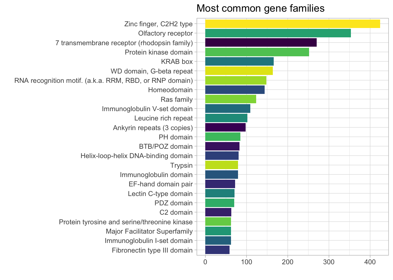
Annotation hub
The Annotation hub is a meta resource for accessing annotation databases. It can be challenging to navigate the Annotation hub if you don’t know what you’re looking for. In the following example, I connect to the hub and then use subset to filter for human genome annotations. I then show a couple of ways to explore the annotation resources, filter the available content and extract data.
ah <- AnnotationHub()
ah <- subset(ah, species == "Homo sapiens")

unique(ah$dataprovider) %>%
  head(10) # Ahub annotation data providers
## [1] "UCSC" "Ensembl"
## [3] "RefNet" "Inparanoid8"
## [5] "NHLBI" "NIH Pathway Interaction Database"
## [7] "BroadInstitute" "Gencode"
## [9] "MISO, VAST-TOOLS, UCSC" "UWashington"unique(ah$rdataclass) %>%
head(10) # Annotation data types## [1] "GRanges" "data.frame" "Inparanoid8Db" "TwoBitFile"
## [5] "ChainFile" "SQLiteConnection" "biopax" "BigWigFile"
## [9] "list" "TxDb"mcols(ah) %>%
head(10) # Provides a DataFrame## DataFrame with 10 rows and 15 columns
## title dataprovider species taxonomyid genome
## <character> <character> <character> <integer> <character>
## AH5012 Chromosome Band UCSC Homo sapiens 9606 hg19
## AH5013 STS Markers UCSC Homo sapiens 9606 hg19
## AH5014 FISH Clones UCSC Homo sapiens 9606 hg19
## AH5015 Recomb Rate UCSC Homo sapiens 9606 hg19
## AH5016 ENCODE Pilot UCSC Homo sapiens 9606 hg19
## AH5017 Map Contigs UCSC Homo sapiens 9606 hg19
## AH5018 Assembly UCSC Homo sapiens 9606 hg19
## AH5019 GRC Map Contigs UCSC Homo sapiens 9606 hg19
## AH5020 Publications UCSC Homo sapiens 9606 hg19
## AH5021 BAC End Pairs UCSC Homo sapiens 9606 hg19
## description coordinate_1_based maintainer
## <character> <integer> <character>
## AH5012 GRanges object from .. 1 Marc Carlson <mcarls..
## AH5013 GRanges object from .. 1 Marc Carlson <mcarls..
## AH5014 GRanges object from .. 1 Marc Carlson <mcarls..
## AH5015 GRanges object from .. 1 Marc Carlson <mcarls..
## AH5016 GRanges object from .. 1 Marc Carlson <mcarls..
## AH5017 GRanges object from .. 1 Marc Carlson <mcarls..
## AH5018 GRanges object from .. 1 Marc Carlson <mcarls..
## AH5019 GRanges object from .. 1 Marc Carlson <mcarls..
## AH5020 GRanges object from .. 1 Marc Carlson <mcarls..
## AH5021 GRanges object from .. 1 Marc Carlson <mcarls..
## rdatadateadded preparerclass tags
## <character> <character> <list>
## AH5012 2013-03-26 UCSCFullTrackImportP.. cytoBand,UCSC,track,...
## AH5013 2013-03-26 UCSCFullTrackImportP.. stsMap,UCSC,track,...
## AH5014 2013-03-26 UCSCFullTrackImportP.. fishClones,UCSC,track,...
## AH5015 2013-03-26 UCSCFullTrackImportP.. recombRate,UCSC,track,...
## AH5016 2013-03-26 UCSCFullTrackImportP.. encodeRegions,UCSC,track,...
## AH5017 2013-03-26 UCSCFullTrackImportP.. ctgPos,UCSC,track,...
## AH5018 2013-03-26 UCSCFullTrackImportP.. gold,UCSC,track,...
## AH5019 2013-03-26 UCSCFullTrackImportP.. ctgPos2,UCSC,track,...
## AH5020 2013-03-26 UCSCFullTrackImportP.. pubs,UCSC,track,...
## AH5021 2013-03-26 UCSCFullTrackImportP.. bacEndPairs,UCSC,track,...
## rdataclass rdatapath sourceurl sourcetype
## <character> <character> <character> <character>
## AH5012 GRanges goldenpath/hg19/data.. rtracklayer://hgdown.. UCSC track
## AH5013 GRanges goldenpath/hg19/data.. rtracklayer://hgdown.. UCSC track
## AH5014 GRanges goldenpath/hg19/data.. rtracklayer://hgdown.. UCSC track
## AH5015 GRanges goldenpath/hg19/data.. rtracklayer://hgdown.. UCSC track
## AH5016 GRanges goldenpath/hg19/data.. rtracklayer://hgdown.. UCSC track
## AH5017 GRanges goldenpath/hg19/data.. rtracklayer://hgdown.. UCSC track
## AH5018 GRanges goldenpath/hg19/data.. rtracklayer://hgdown.. UCSC track
## AH5019 GRanges goldenpath/hg19/data.. rtracklayer://hgdown.. UCSC track
## AH5020 GRanges goldenpath/hg19/data.. rtracklayer://hgdown.. UCSC track
## AH5021 GRanges goldenpath/hg19/data.. rtracklayer://hgdown.. UCSC trackgrs <- query(ah, pattern = "GRanges") # filter for annotations that are GRanges
grs## AnnotationHub with 14214 records
## # snapshotDate(): 2021-05-18
## # $dataprovider: BroadInstitute, UCSC, Ensembl, Gencode, GENCODE, EMBL-EBI, ...
## # $species: Homo sapiens
## # $rdataclass: GRanges, data.frame, DNAStringSet, GRanges
## # additional mcols(): taxonomyid, genome, description,
## # coordinate_1_based, maintainer, rdatadateadded, preparerclass, tags,
## # rdatapath, sourceurl, sourcetype
## # retrieve records with, e.g., 'object[["AH5012"]]'
##
## title
## AH5012 | Chromosome Band
## AH5013 | STS Markers
## AH5014 | FISH Clones
## AH5015 | Recomb Rate
## AH5016 | ENCODE Pilot
## ... ...
## AH80075 | Homo_sapiens.GRCh38.100.chr.gtf
## AH80076 | Homo_sapiens.GRCh38.100.chr_patch_hapl_scaff.gtf
## AH80077 | Homo_sapiens.GRCh38.100.gtf
## AH95565 | CTCF_hg19.RData
## AH95566 | CTCF_hg38.RData#display(ah)
# Example of extracting data from the query results
res <- grs[[1]] # extracting the first annotation resource
head(res)## UCSC track 'cytoBand'
## UCSCData object with 6 ranges and 1 metadata column:
## seqnames ranges strand | name
## <Rle> <IRanges> <Rle> | <character>
## [1] chr1 1-2300000 * | p36.33
## [2] chr1 2300001-5400000 * | p36.32
## [3] chr1 5400001-7200000 * | p36.31
## [4] chr1 7200001-9200000 * | p36.23
## [5] chr1 9200001-12700000 * | p36.22
## [6] chr1 12700001-16200000 * | p36.21
## -------
## seqinfo: 93 sequences (1 circular) from hg19 genomeI am excited to move forward in this series of posts on bioinformatics and will definitely be revisiting many of the packages that I’ve discussed so far. Up to this point, we have focused on reference genome sequence ranges, sequence extraction, genomic visualization and annotation. In future posts, I hope to incorporate genomic data analysis using experimental data. Until then, stay safe and keep coding!
Gabriel Mednick, PhD
Data scientist, biochemist, computational biologist, educator, life enthusiast