Loan data analysis
Loan Data
This dataset consists of data from almost 10,000 borrowers that took loans with some paid back and others still in progress. It was extracted from lendingclub.com which is an organization that connects borrowers with investors.
Understand your data
| Variable | class | description |
|---|---|---|
| credit_policy | numeric | 1 if the customer meets the credit underwriting criteria; 0 otherwise. |
| purpose | character | The purpose of the loan. |
| int_rate | numeric | The interest rate of the loan (more risky borrowers are assigned higher interest rates). |
| installment | numeric | The monthly installments owed by the borrower if the loan is funded. |
| log_annual_inc | numeric | The natural log of the self-reported annual income of the borrower. |
| dti | numeric | The debt-to-income ratio of the borrower (amount of debt divided by annual income). |
| fico | numeric | The FICO credit score of the borrower. |
| days_with_cr_line | numeric | The number of days the borrower has had a credit line. |
| revol_bal | numeric | The borrower’s revolving balance (amount unpaid at the end of the credit card billing cycle). |
| revol_util | numeric | The borrower’s revolving line utilization rate (the amount of the credit line used relative to total credit available). |
| inq_last_6mths | numeric | The borrower’s number of inquiries by creditors in the last 6 months. |
| delinq_2yrs | numeric | The number of times the borrower had been 30+ days past due on a payment in the past 2 years. |
| pub_rec | numeric | The borrower’s number of derogatory public records. |
| not_fully_paid | numeric | 1 if the loan is not fully paid; 0 otherwise. |
Load packages
# install.packages('ggridges')
# install.packages('patchwork')
# install.packages('gt')
# install.packages('xgboost')
# install.packages('ranger')
# install.packages('vip')
# install.packages('usemodels')
# install.packages('GGally')
# install.packages('doParallel')
# install.packages('glmnet')
library(skimr)
library(tidyverse)
library(tidymodels)
library(scales)
library(ggridges)
library(patchwork)
library(gt)
library(xgboost)
library(ranger)
library(vip)
library(usemodels)
library(GGally)
library(glmnet)
doParallel::registerDoParallel()
theme_set(theme_light())
Load the Data
loans <- readr::read_csv('loans.csv.gz')Exploratory data analysis
As a strong visual learner, it helps me to see the data in both table and plot formats. Let’s get started by looking at a few the summary statistics generated from the skimr::skim() combined with summary(). I will also use glimpse() to get a concise view of the data names, data types and the first few entries.
loans %>%
  skim() %>%
  select(-(numeric.p0:numeric.p100)) %>%
  select(-(complete_rate)) %>%
summary()| Name | Piped data |
| Number of rows | 9578 |
| Number of columns | 14 |
| _______________________ | |
| Column type frequency: | |
| character | 1 |
| numeric | 13 |
| ________________________ | |
| Group variables | None |
loans %>%
  glimpse()
## Rows: 9,578
## Columns: 14
## $ credit_policy <dbl> 1, 1, 1, 1, 1, 1, 1, 1, 1, 1, 1, 1, 1, 1, 1, 1, 1, 1…
## $ purpose <chr> "debt_consolidation", "credit_card", "debt_consolida…
## $ int_rate <dbl> 0.1189, 0.1071, 0.1357, 0.1008, 0.1426, 0.0788, 0.14…
## $ installment <dbl> 829.10, 228.22, 366.86, 162.34, 102.92, 125.13, 194.…
## $ log_annual_inc <dbl> 11.350407, 11.082143, 10.373491, 11.350407, 11.29973…
## $ dti <dbl> 19.48, 14.29, 11.63, 8.10, 14.97, 16.98, 4.00, 11.08…
## $ fico <dbl> 737, 707, 682, 712, 667, 727, 667, 722, 682, 707, 67…
## $ days_with_cr_line <dbl> 5639.958, 2760.000, 4710.000, 2699.958, 4066.000, 61…
## $ revol_bal <dbl> 28854, 33623, 3511, 33667, 4740, 50807, 3839, 24220,…
## $ revol_util <dbl> 52.1, 76.7, 25.6, 73.2, 39.5, 51.0, 76.8, 68.6, 51.1…
## $ inq_last_6mths <dbl> 0, 0, 1, 1, 0, 0, 0, 0, 1, 1, 2, 2, 0, 0, 0, 1, 0, 1…
## $ delinq_2yrs <dbl> 0, 0, 0, 0, 1, 0, 0, 0, 0, 0, 0, 1, 0, 1, 0, 0, 0, 0…
## $ pub_rec <dbl> 0, 0, 0, 0, 0, 0, 1, 0, 0, 0, 1, 0, 0, 0, 0, 0, 0, 0…
## $ not_fully_paid <dbl> 0, 0, 0, 0, 0, 0, 1, 1, 0, 0, 0, 0, 0, 0, 0, 0, 0, 0…loans %>%
head() %>%
gt() %>%
tab_header(title = md("**First 6 rows of loan data from lendingclub.com**")) %>%
tab_options(container.height = 400,
container.overflow.y = TRUE,
heading.background.color = "#21908CFF",
table.width = "75%",
column_labels.background.color = "black",
table.font.color = "black") %>%
tab_style(style = list(cell_fill(color = "#35B779FF")),
locations = cells_body())| First 6 rows of loan data from lendingclub.com | |||||||||||||
|---|---|---|---|---|---|---|---|---|---|---|---|---|---|
| credit_policy | purpose | int_rate | installment | log_annual_inc | dti | fico | days_with_cr_line | revol_bal | revol_util | inq_last_6mths | delinq_2yrs | pub_rec | not_fully_paid |
| 1 | debt_consolidation | 0.1189 | 829.10 | 11.35041 | 19.48 | 737 | 5639.958 | 28854 | 52.1 | 0 | 0 | 0 | 0 |
| 1 | credit_card | 0.1071 | 228.22 | 11.08214 | 14.29 | 707 | 2760.000 | 33623 | 76.7 | 0 | 0 | 0 | 0 |
| 1 | debt_consolidation | 0.1357 | 366.86 | 10.37349 | 11.63 | 682 | 4710.000 | 3511 | 25.6 | 1 | 0 | 0 | 0 |
| 1 | debt_consolidation | 0.1008 | 162.34 | 11.35041 | 8.10 | 712 | 2699.958 | 33667 | 73.2 | 1 | 0 | 0 | 0 |
| 1 | credit_card | 0.1426 | 102.92 | 11.29973 | 14.97 | 667 | 4066.000 | 4740 | 39.5 | 0 | 1 | 0 | 0 |
| 1 | credit_card | 0.0788 | 125.13 | 11.90497 | 16.98 | 727 | 6120.042 | 50807 | 51.0 | 0 | 0 | 0 | 0 |
The loan data consists of one character variable (‘purpose’ = loan type) and 13 numeric variables. Let’s use geom_col() to plot the number of times each loan type is represented in the data.
loans %>%
  count(purpose) %>%
  mutate(purpose = fct_reorder(purpose, n)) %>%
  ggplot(aes(n, purpose, fill = purpose)) +
  geom_col() +
  labs(title = 'Loan count by type',
       x = 'Count',
       y = '') +
  theme(legend.position = 'none') +
  scale_fill_viridis_d()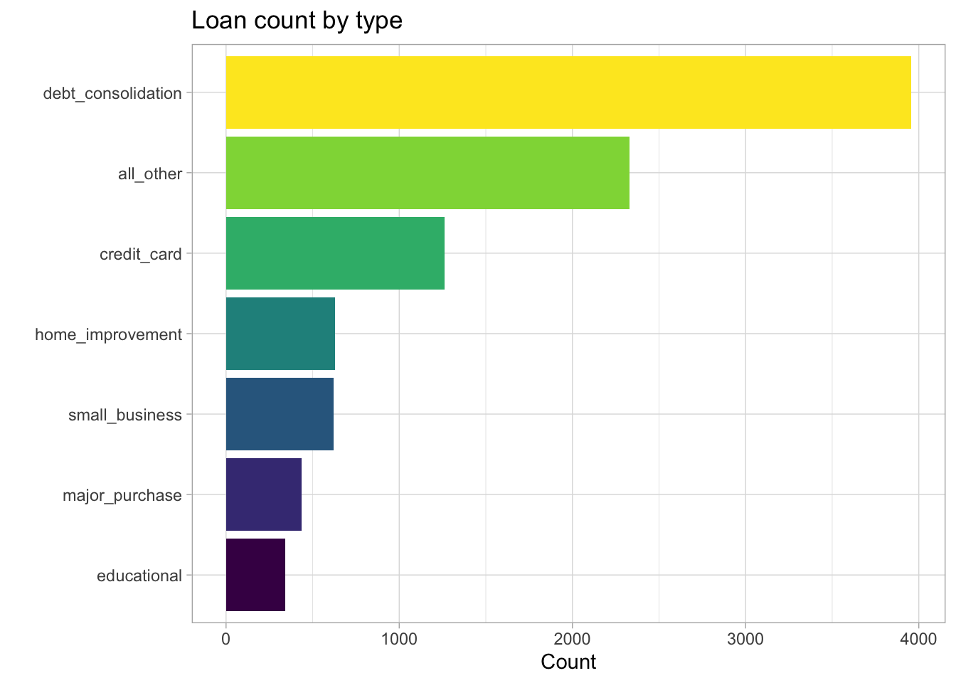
Figure 1: Counts of each loan type
Numeric variables can be viewed as count distributions using geom_histogram(). Here, I use the gather() function to reshape the data into a long format and then facet_wrap() is used to display each histogram in a single figure.
loans[c(3:13)] %>%
  mutate(log_revol_bal = log(revol_bal)) %>%
  select(-revol_bal) %>%
  gather() %>%
  ggplot(aes(value, fill = key)) +
  geom_histogram(alpha = 0.7) +
  facet_wrap(~key, scales = 'free') +
  labs(title = 'Count distributions for numeric variables') +
  theme(legend.position = 'none')
## Warning: Removed 321 rows containing non-finite values (stat_bin).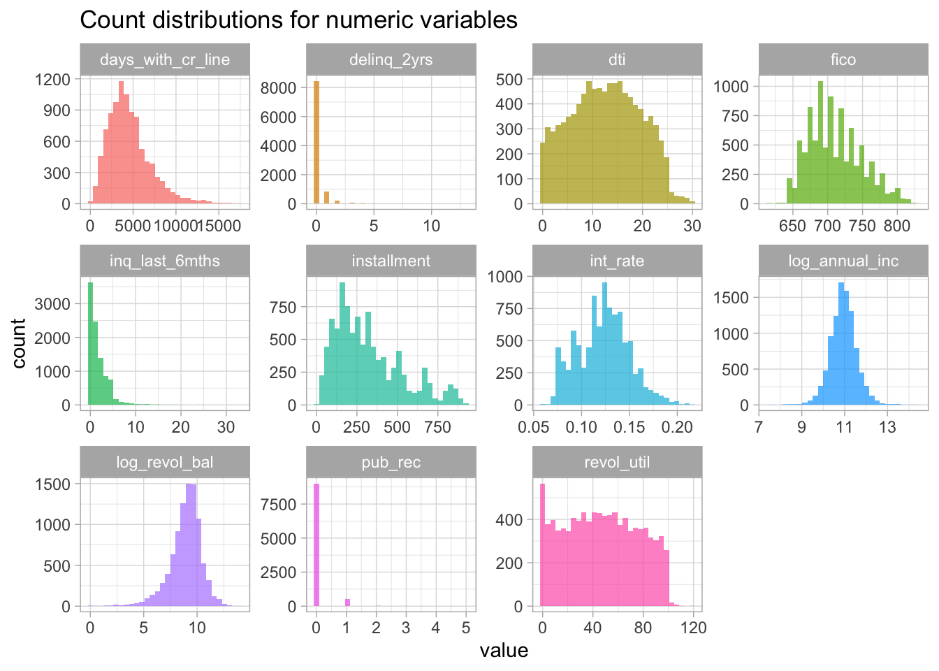
Figure 2: Histograms of all numeric variables
The credit_policy and not_fully_paid variables (not shown above) are better represented as factors. They can be converted using the recode_factor() function. Let’s convert them to factors and explore their distributions with geom_boxplot().
loans <- loans %>%
  mutate(not_fully_paid = recode_factor(not_fully_paid, '1' = 'No', '0' = 'Yes'),
         credit_policy = recode_factor(credit_policy, '1' = 'pass', '0' = 'fail'),
         purpose = factor(purpose))
loans %>%
select(-c(12:13)) %>%
pivot_longer(!c(credit_policy, purpose, not_fully_paid)) %>%
#filter(name != 'revol_bal') %>%
ggplot(aes(value, fill = not_fully_paid)) +
geom_boxplot() +
facet_wrap(~name, scales = 'free') +
labs(title = "Comparing loan payment status across other variables",
x = "") +
guides(fill = guide_legend(reverse=TRUE))
Figure 3: Boxplots comparing fully paid and not fully paid across numeric variables
library(ggpubr)
loans %>%
  select(c(1:10)) %>%
  pivot_longer(!c(purpose, credit_policy)) %>%
  filter(name != 'revol_bal') %>%
  ggplot(aes(value, fill = credit_policy)) +
  geom_boxplot()  +
  facet_wrap(~name, scales = 'free') +
  labs(title = "Comparing credit policy across other variables",
       x = "") +
  guides(fill = guide_legend(reverse=TRUE))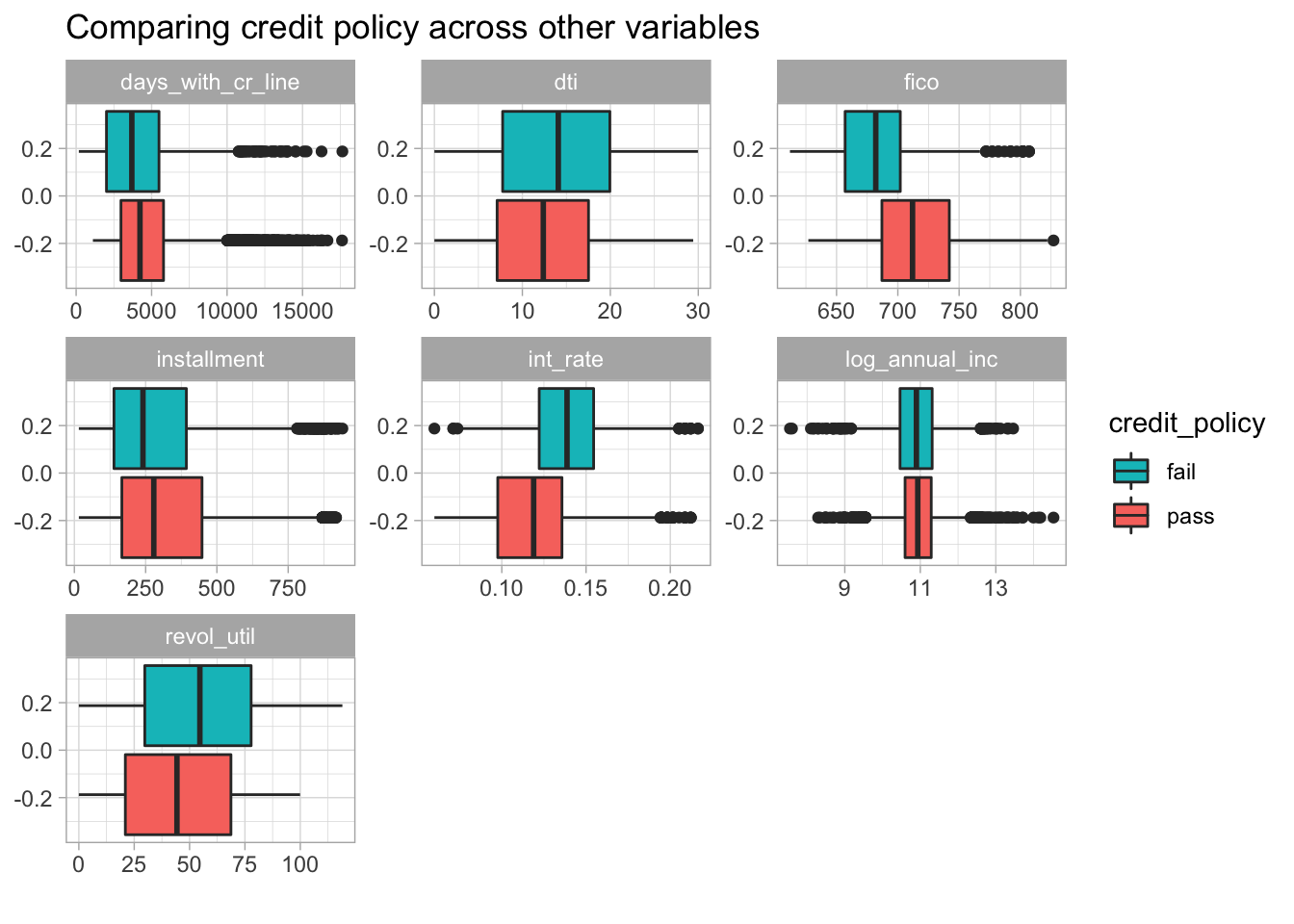
Figure 4: Boxplots of numeric features across credit risk assessment
Loan type can also be viewed with geom_boxplot() but the categories get a little crowded.
loans %>%
  select(-c(9, 11:13)) %>%
  pivot_longer(!c(credit_policy, purpose, not_fully_paid)) %>%
  #filter(name != 'revol_bal') %>%
  ggplot(aes(value, fill = purpose)) +
  geom_boxplot()  +
  facet_wrap(~name, scales = 'free') +
  labs(title = "Comparing loan payment status across other variables",
       x = "") +
  guides(fill = guide_legend(reverse=TRUE))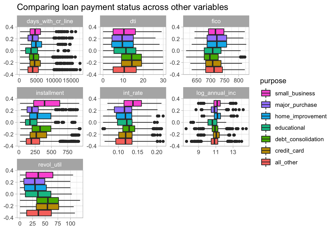
Figure 5: Boxplots of numeric features across loan types
The geom_density_ridges() function from the ggridges package is an alternative way to view a numeric distribution across multiple categories.
a <- loans %>%
  add_count(purpose) %>%
  mutate(purpose = fct_reorder(purpose, n)) %>%
  group_by(purpose) %>%
  ggplot(aes(int_rate, purpose, fill = purpose)) +
  geom_density_ridges() +
  labs(title = 'Density of the interest rate by loan purpose',
       x= 'Interest rate',
       y= '') +
  theme(legend.position = 'none') +
  scale_fill_viridis_d(alpha = 0.8) +
  theme(panel.grid.minor = element_blank(), panel.border = element_blank())

b <- loans %>%
  add_count(purpose) %>%
  mutate(purpose = fct_reorder(purpose, n)) %>%
  group_by(purpose) %>%
  ggplot(aes(dti, purpose, fill = purpose)) +
  geom_density_ridges() +
  # scale_y_discrete(expand = c(0.01, 0)) +
  # scale_x_continuous(expand = c(0.01, 0)) +
  #theme_ridges() +
  labs(title = 'Density of the debt-to-income ratio by loan purpose',
       x= 'dti',
       y= '') +
  theme(legend.position = 'none') +
  scale_fill_viridis_d(alpha = 0.8) +
  theme(panel.grid.minor = element_blank(), panel.border = element_blank())

(a  / b)
## Picking joint bandwidth of 0.00625## Picking joint bandwidth of 1.57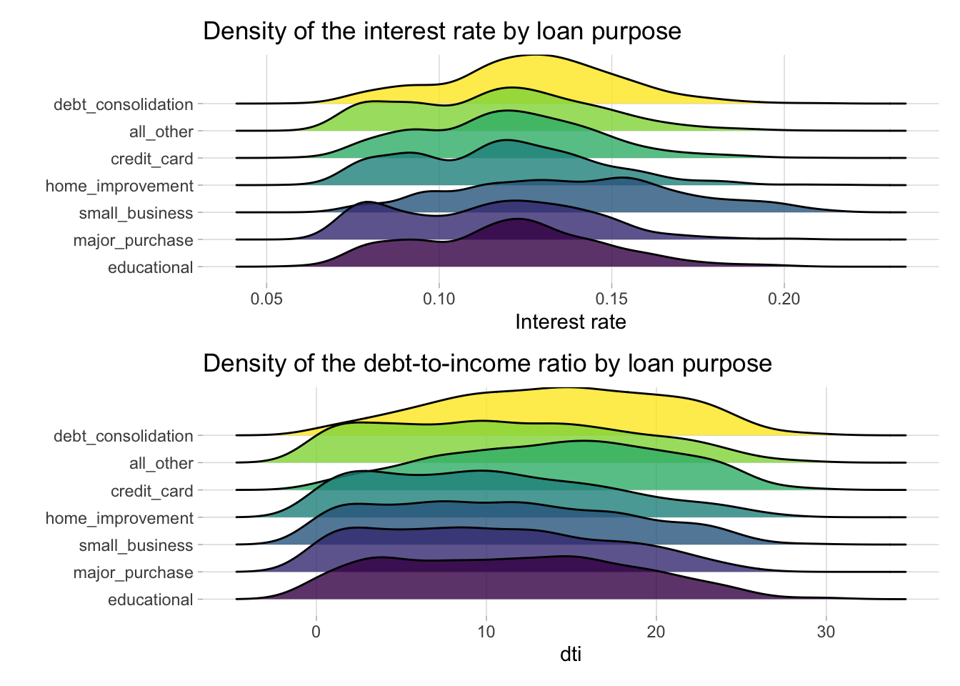
Figure 6: Density plots of interest rate and debt-to-interest across loan types
c <- loans %>%
  add_count(purpose) %>%
  mutate(purpose = fct_reorder(purpose, n)) %>%
  group_by(purpose) %>%
  ggplot(aes(revol_util, purpose, fill = purpose)) +
  geom_density_ridges() +
  labs(title = 'Density of the revol_util by loan purpose',
       x= 'revol_util',
       y= '') +
  theme(legend.position = 'none') +
  scale_fill_viridis_d(alpha = 0.8) +
  theme(panel.grid.minor = element_blank(), panel.border = element_blank())

d <- loans %>%
  add_count(purpose) %>%
  mutate(purpose = fct_reorder(purpose, n)) %>%
  group_by(purpose) %>%
  ggplot(aes(installment, purpose, fill = purpose)) +
  geom_density_ridges() +
  labs(title = 'Density of the installment by loan purpose',
       x= 'installment',
       y= '') +
  theme(legend.position = 'none') +
  scale_fill_viridis_d(alpha = 0.8) +
  theme(panel.grid.minor = element_blank(), panel.border = element_blank())

(c / d)
## Picking joint bandwidth of 6.58## Picking joint bandwidth of 41.9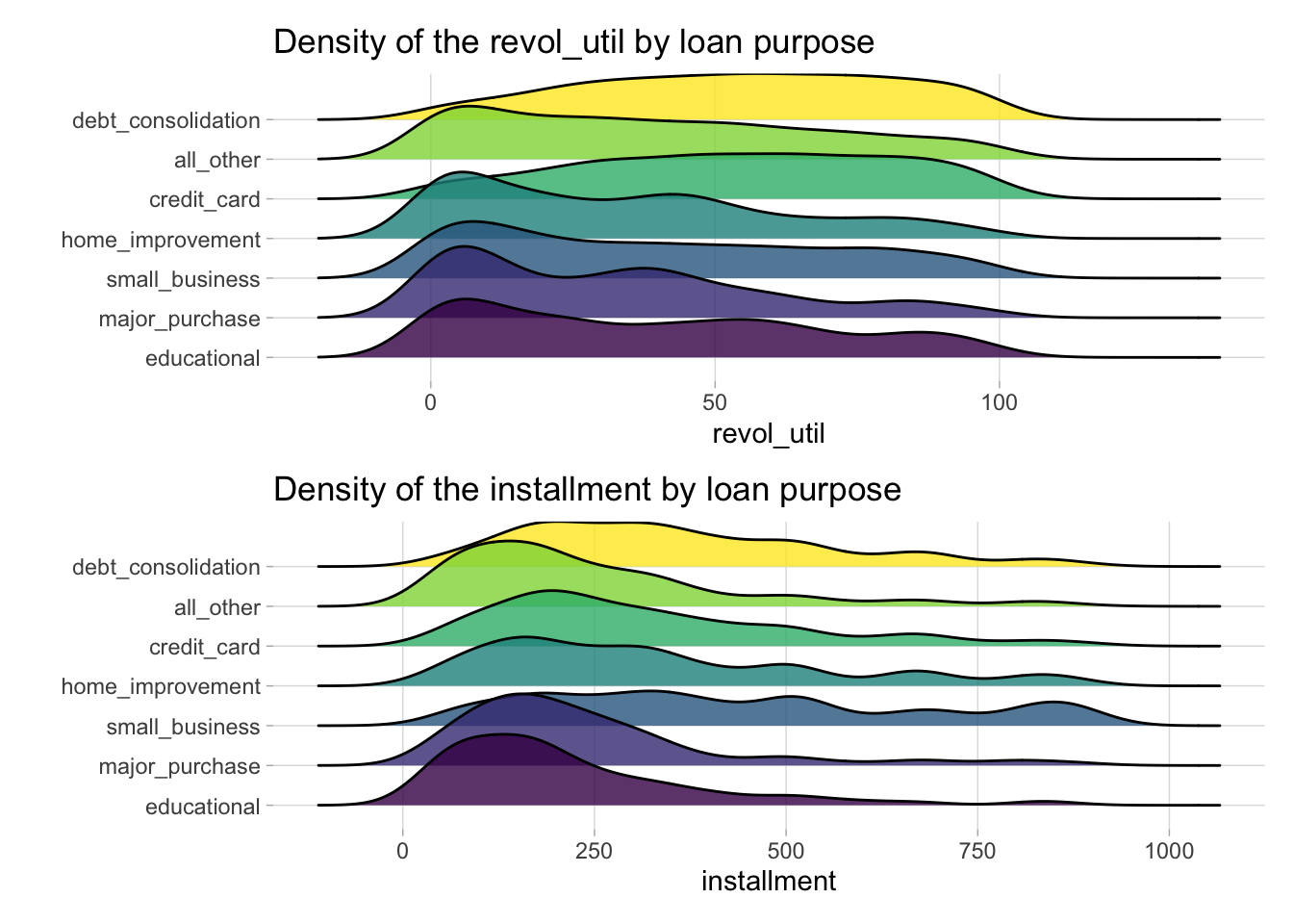
Figure 7: Density plots of revolving line utilization rate and installment variables across loan types
The ggpairs() function from the GGally package allows us to summarize correlation values between our variables.
loans[c(3:8, 10)] %>%
  sample_n(size = 500) %>%
  ggpairs()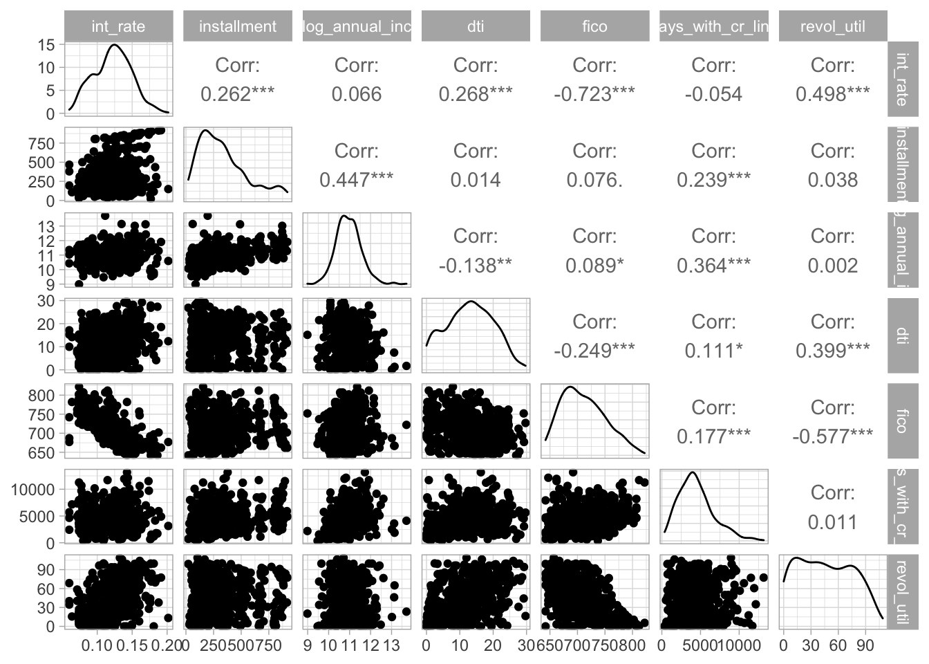
Figure 8: Correlation values between numeric variables
Modeling challenges
Now that we have a feel for our data, let’s create some models!
- Create a model that predicts the loan type (purpose)
- Create model that predicts whether the loan has been payed back (not_fully_paid)
- Create a model that predicts whether the loanee meets the accepted level of risk (credit_policy)
Splitting the data
The data is split into training and test sets using the default (prop = 0.75) split. 5-fold cross validation is used to create resamples from the training set.
split <- loans %>% initial_split()
train <- training(split) %>% sample_n(size = 500)
test <- testing(split)

resamps <- vfold_cv(train, v = 5)
Predicting loan type
To predict the loan type we will need to build a multiclass classification model. I am going to try three different models and compare the results to determine which model has the best predictive power.
Model 1: Xgboost
#usemodels::use_xgboost(purpose ~ ., data = train)
xgboost_recipe <-
  recipe(formula = purpose ~ ., data = train) %>%
  step_novel(all_nominal(), -all_outcomes()) %>%
  step_dummy(all_nominal(), -all_outcomes(), one_hot = TRUE) %>%
  step_zv(all_predictors())

xgboost_spec <-
  boost_tree(
    trees = 1000,
    tree_depth = tune(),
    min_n = tune(),
    mtry = tune(),
    sample_size = tune(),
    learn_rate = tune()
  ) %>%
  set_engine("xgboost") %>%
  set_mode("classification")

xgboost_workflow <-
  workflow() %>%
  add_recipe(xgboost_recipe) %>%
  add_model(xgboost_spec)

# xgboost_grid_1 <- grid_regular(
#   parameters(xgboost_spec),
#   levels = 3 )

# xgboost_grid_2 <- grid_regular(
#   tree_depth(c(5L, 10L)),
#     min_n(c(10L, 40L)),
#     mtry(c(5L, 10L)),
#     learn_rate(c(-2, -1)),
#   sample_size=20
# )

set.seed(8390)
xgboost_tune <-
  tune_grid(xgboost_workflow, resamples = resamps, grid = 20)
## i Creating pre-processing data to finalize unknown parameter: mtryxgboost_tune %>%
autoplot()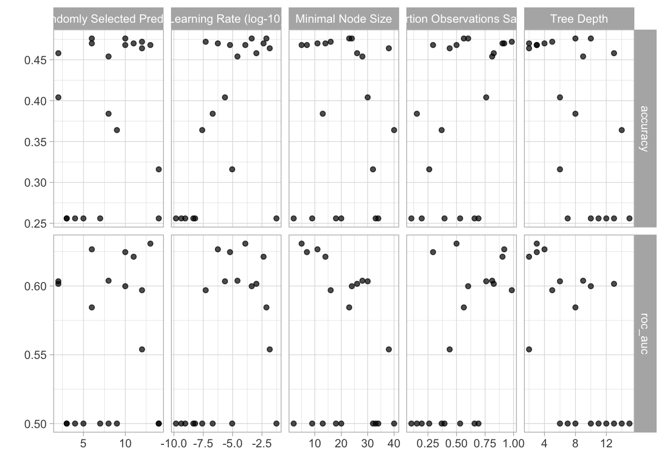
xg_best_params <- xgboost_tune %>%
select_best(metric = 'accuracy')
xg_best_spec <- xgboost_spec %>%
finalize_model(xg_best_params)
xg_final_fit <- workflow() %>%
add_recipe(xgboost_recipe) %>%
add_model(xg_best_spec) %>%
last_fit(split = split)
xg_final_fit %>%
collect_metrics()## # A tibble: 2 × 4
## .metric .estimator .estimate .config
## <chr> <chr> <dbl> <chr>
## 1 accuracy multiclass 0.489 Preprocessor1_Model1
## 2 roc_auc hand_till 0.695 Preprocessor1_Model1Model 2: Random forest
# usemodels::use_ranger(purpose ~ ., data = train)
ranger_recipe <-
recipe(formula = purpose ~ ., data = train)
ranger_spec <-
rand_forest(mtry = tune(),
min_n = tune(),
trees = 1000) %>%
set_mode("classification") %>%
set_engine("ranger")
rand_forest(mode = "classification") %>%
set_engine("ranger", importance = "impurity") %>%
fit(purpose ~ .,
data = train) %>%
vip::vip(geom = 'point',
aesthetics = list(color = 'midnightblue', size = 4)) +
labs(title = 'test')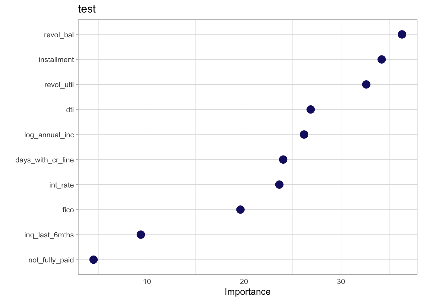
ranger_workflow <-
workflow() %>%
add_recipe(ranger_recipe) %>%
add_model(ranger_spec)
# ranger_grid <- grid_regular(
# parameters(ranger_spec),
# mtry(range = c(10, 30)),
# min_n(range = c(2, 8)),
# levels = 3)
set.seed(57341)
ranger_tune <-
tune_grid(ranger_workflow,
resamples = resamps,
grid = 20)## i Creating pre-processing data to finalize unknown parameter: mtryranger_tune %>%
autoplot()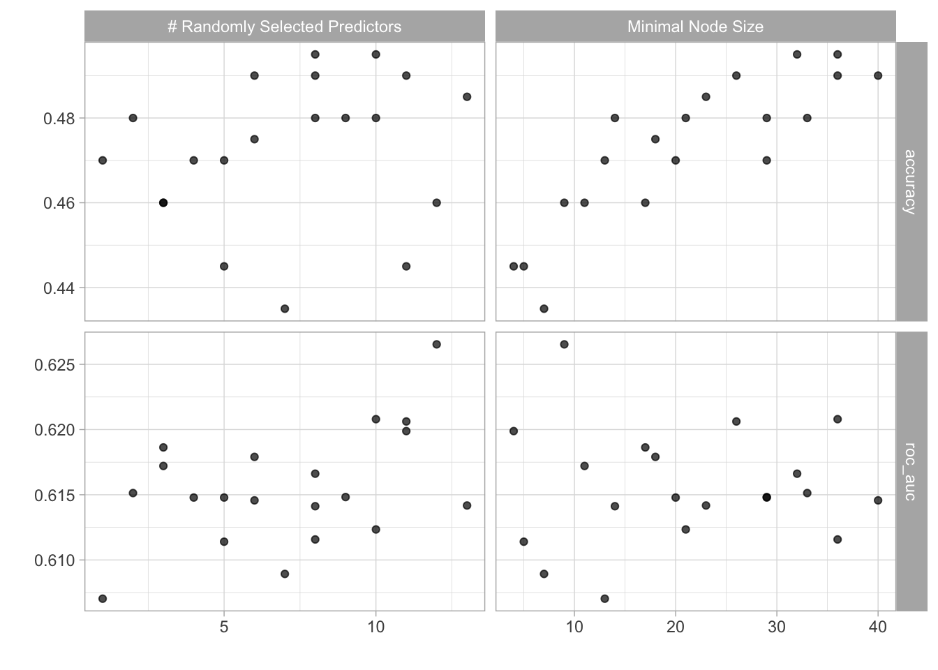
rf_best_params <- ranger_tune %>%
select_best(metric = 'accuracy')
rf_best_spec <- ranger_spec %>%
finalize_model(rf_best_params)
rf_final_fit <- workflow() %>%
add_recipe(ranger_recipe) %>%
add_model(rf_best_spec) %>%
last_fit(split = split)
rf_final_fit %>%
collect_metrics()## # A tibble: 2 × 4
## .metric .estimator .estimate .config
## <chr> <chr> <dbl> <chr>
## 1 accuracy multiclass 0.489 Preprocessor1_Model1
## 2 roc_auc hand_till 0.693 Preprocessor1_Model1Model 3: K-nearest neighbors
#usemodels::use_kknn(purpose ~ ., data = train)
kknn_recipe <-
recipe(formula = purpose ~ ., data = train) %>%
step_novel(all_nominal(), -all_outcomes()) %>%
step_dummy(all_nominal(), -all_outcomes()) %>%
step_zv(all_predictors()) %>%
step_normalize(all_predictors(), -all_nominal())
kknn_spec <-
nearest_neighbor(neighbors = tune(), weight_func = tune()) %>%
set_mode("classification") %>%
set_engine("kknn")
kknn_workflow <-
workflow() %>%
add_recipe(kknn_recipe) %>%
add_model(kknn_spec)
knn_grid <- grid_regular(
parameters(kknn_spec),
mtry(range = c(10, 30)),
levels = 5)
set.seed(78590)
kknn_tune <-
tune_grid(kknn_workflow,
resamples = resamps,
grid = knn_grid)
kknn_tune %>%
autoplot()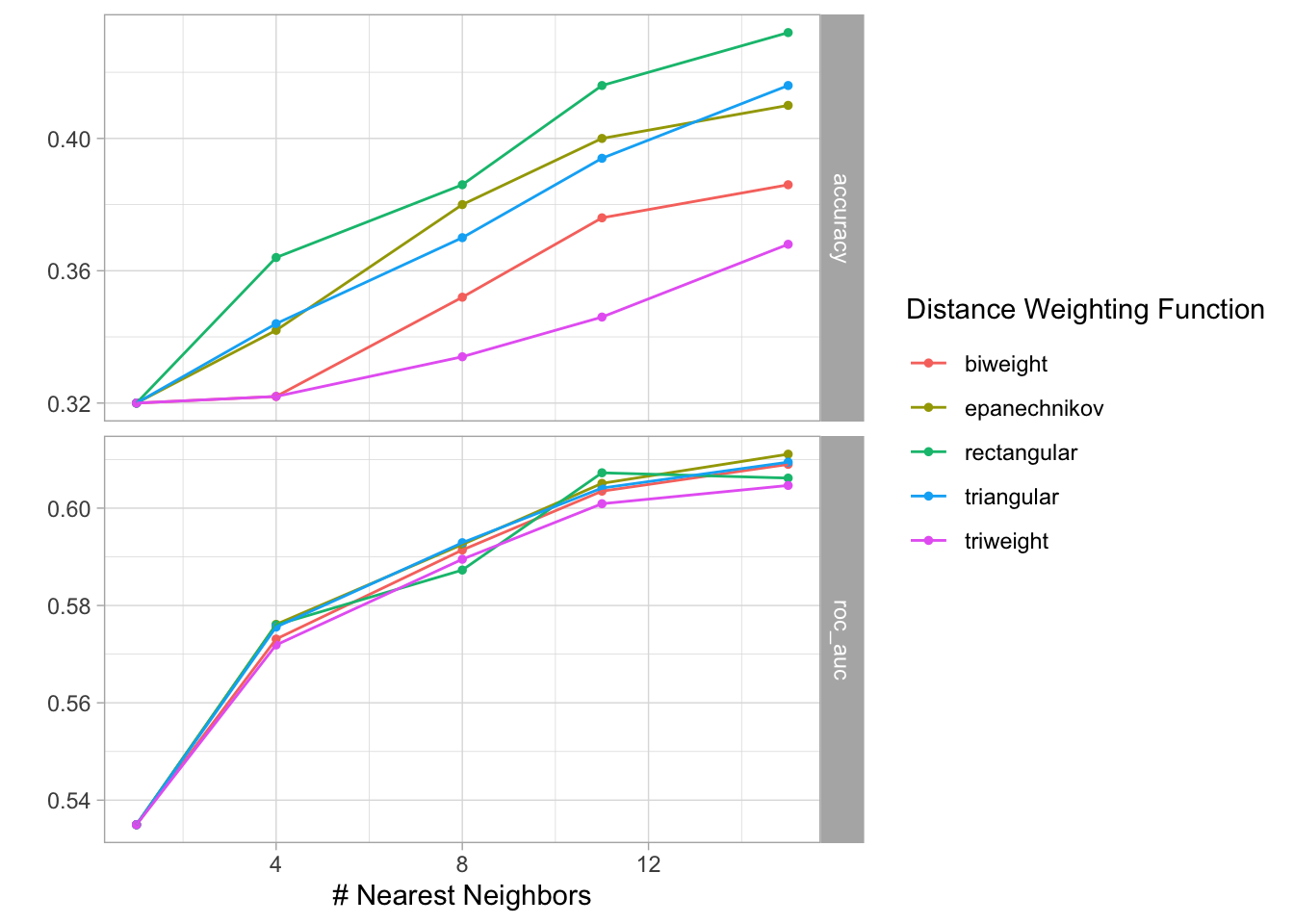
knn_best_params <- kknn_tune %>%
select_best(metric = 'accuracy')
knn_best_spec <- kknn_spec %>%
finalize_model(knn_best_params)
knn_final_fit <- workflow() %>%
add_recipe(kknn_recipe) %>%
add_model(knn_best_spec) %>%
last_fit(split = split)
knn_final_fit %>%
collect_metrics()## # A tibble: 2 × 4
## .metric .estimator .estimate .config
## <chr> <chr> <dbl> <chr>
## 1 accuracy multiclass 0.445 Preprocessor1_Model1
## 2 roc_auc hand_till 0.623 Preprocessor1_Model1knn_final_fit %>%
collect_predictions()## # A tibble: 2,395 × 12
## id .pred_all_other .pred_credit_ca… .pred_debt_cons… .pred_education…
## <chr> <dbl> <dbl> <dbl> <dbl>
## 1 train/test split 0.2 0.333 0.333 0
## 2 train/test split 0.267 0.133 0.467 0.0667
## 3 train/test split 0.2 0.533 0.0667 0.0667
## 4 train/test split 0.2 0.2 0.4 0
## 5 train/test split 0.0667 0.333 0.267 0.2
## 6 train/test split 0.0667 0.0667 0.667 0.0667
## 7 train/test split 0.267 0.267 0.4 0
## 8 train/test split 0.333 0.0667 0.333 0.0667
## 9 train/test split 0.333 0.0667 0.0667 0.0667
## 10 train/test split 0.467 0.267 0.2 0.0667
## # … with 2,385 more rows, and 7 more variables: .pred_home_improvement <dbl>,
## # .pred_major_purchase <dbl>, .pred_small_business <dbl>, .row <int>,
## # .pred_class <fct>, purpose <fct>, .config <chr>models <- c('xgboost', 'xgboost', 'random forrest', 'random forrest', 'knn', 'knn')
bind_rows(xg_final_fit %>% collect_metrics(), rf_final_fit %>% collect_metrics(), knn_final_fit %>%
collect_metrics()) %>%
mutate(models = models) %>%
select(models, everything(), -.config) %>%
gt() %>%
tab_header(title = 'Model Results') %>%
tab_options(container.height = 400,
container.overflow.y = TRUE,
heading.background.color = "#21908CFF",
table.width = "75%",
column_labels.background.color = "black",
table.font.color = "black") %>%
tab_style(style = list(cell_fill(color = "#35B779FF")),
locations = cells_body())| Model Results | |||
|---|---|---|---|
| models | .metric | .estimator | .estimate |
| xgboost | accuracy | multiclass | 0.4885177 |
| xgboost | roc_auc | hand_till | 0.6949143 |
| random forrest | accuracy | multiclass | 0.4893528 |
| random forrest | roc_auc | hand_till | 0.6930445 |
| knn | accuracy | multiclass | 0.4446764 |
| knn | roc_auc | hand_till | 0.6231237 |
Predicting loan risk status (credit policy)
For the next two models, I will use xgboost.
# #usemodels::use_xgboost(credit_policy ~ ., data = train)
xgboost_recipe <-
recipe(formula = credit_policy ~ ., data = train) %>%
step_novel(all_nominal(), -all_outcomes()) %>%
step_dummy(all_nominal(), -all_outcomes(), one_hot = TRUE) %>%
step_zv(all_predictors())
xgboost_spec <-
boost_tree(trees = tune(), min_n = tune(), tree_depth = tune(), learn_rate = tune(),
loss_reduction = tune(), sample_size = tune()) %>%
set_mode("classification") %>%
set_engine("xgboost")
xgboost_workflow <-
workflow() %>%
add_recipe(xgboost_recipe) %>%
add_model(xgboost_spec)
set.seed(10500)
xgboost_tune <-
tune_grid(xgboost_workflow, resamples = resamps, grid = 10)
xgboost_tune %>%
  autoplot()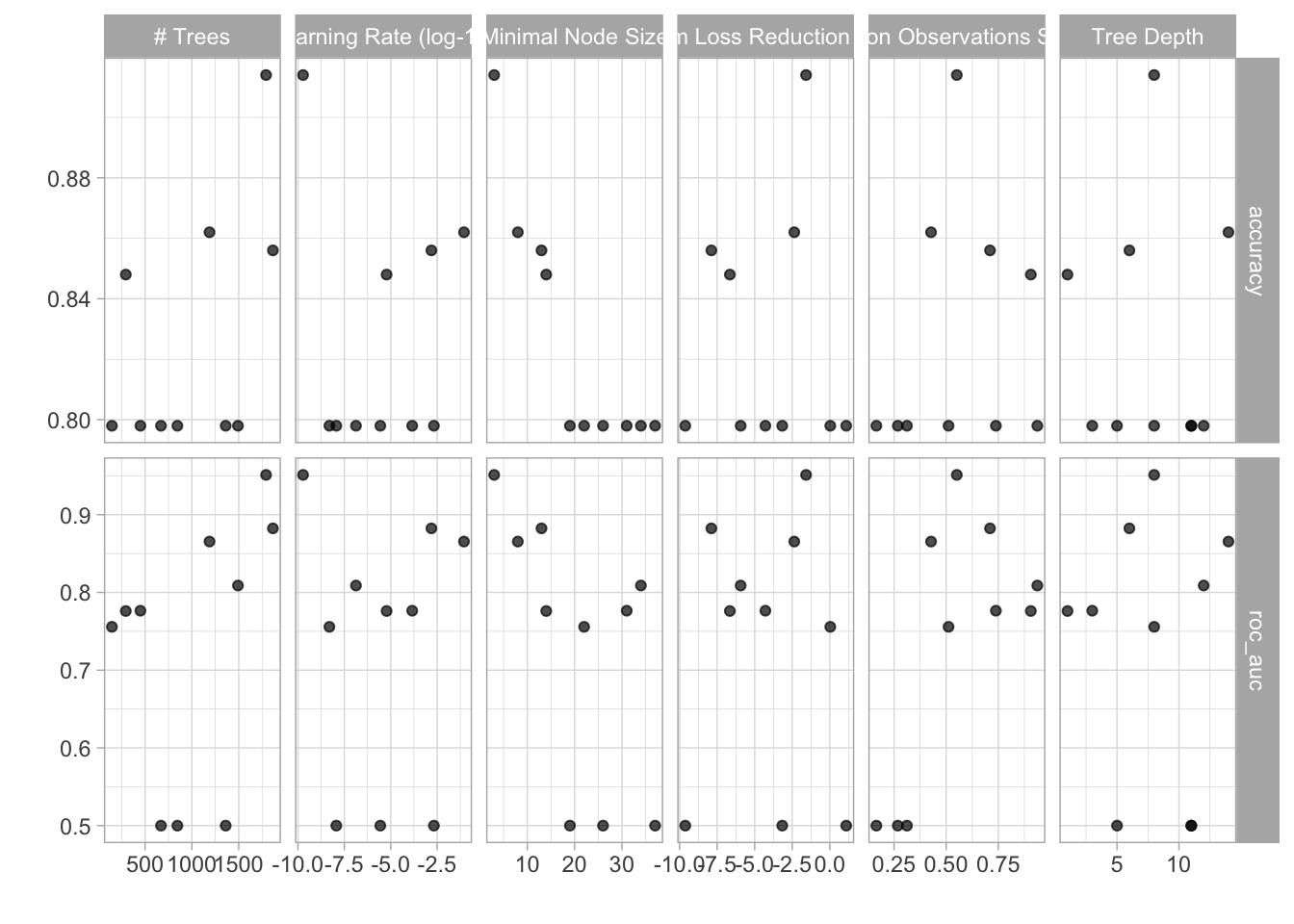
xg_best_params <- xgboost_tune %>%
  select_best(metric = 'accuracy')

xg_best_spec <- xgboost_spec %>%
  finalize_model(xg_best_params)

xg_final_fit <- workflow() %>%
  add_recipe(xgboost_recipe) %>%
  add_model(xg_best_spec) %>%
  last_fit(split = split)

xg_final_fit %>%
collect_metrics() %>%
gt() %>%
tab_header(title = 'Loan risk prediction results') %>%
tab_options(container.height = 400,
container.overflow.y = TRUE,
heading.background.color = "#21908CFF",
table.width = "75%",
column_labels.background.color = "black",
table.font.color = "black") %>%
tab_style(style = list(cell_fill(color = "#35B779FF")),
locations = cells_body())| Loan risk prediction results | |||
|---|---|---|---|
| .metric | .estimator | .estimate | .config |
| accuracy | binary | 0.9787056 | Preprocessor1_Model1 |
| roc_auc | binary | 0.9833877 | Preprocessor1_Model1 |
Predicting loan payment status
#usemodels::use_xgboost(not_fully_paid ~ ., data = train)

xgboost_recipe <-
  recipe(formula = not_fully_paid ~ ., data = train) %>%
  step_string2factor(purpose, not_fully_paid) %>%
  step_novel(all_nominal(), -all_outcomes()) %>%
  step_dummy(all_nominal(), -all_outcomes(), one_hot = TRUE) %>%
  step_zv(all_predictors())

xgboost_spec <-
  boost_tree(trees = tune(), learn_rate = tune()) %>%
  set_mode("classification") %>%
  set_engine("xgboost")

boost_tree(mode = "classification") %>%
  set_engine("xgboost", importance = "impurity") %>%
  fit(purpose ~ .,
      data = train) %>%
  vip::vip(geom = 'point',
           aesthetics = list(color = 'midnightblue', size = 4)) +
  labs(title = 'test')
## [10:20:02] WARNING: amalgamation/../src/learner.cc:573:
## Parameters: { "importance" } might not be used.
##
## This may not be accurate due to some parameters are only used in language bindings but
## passed down to XGBoost core. Or some parameters are not used but slip through this
## verification. Please open an issue if you find above cases.
##
##
## [10:20:02] WARNING: amalgamation/../src/learner.cc:1095: Starting in XGBoost 1.3.0, the default evaluation metric used with the objective 'multi:softprob' was changed from 'merror' to 'mlogloss'. Explicitly set eval_metric if you'd like to restore the old behavior.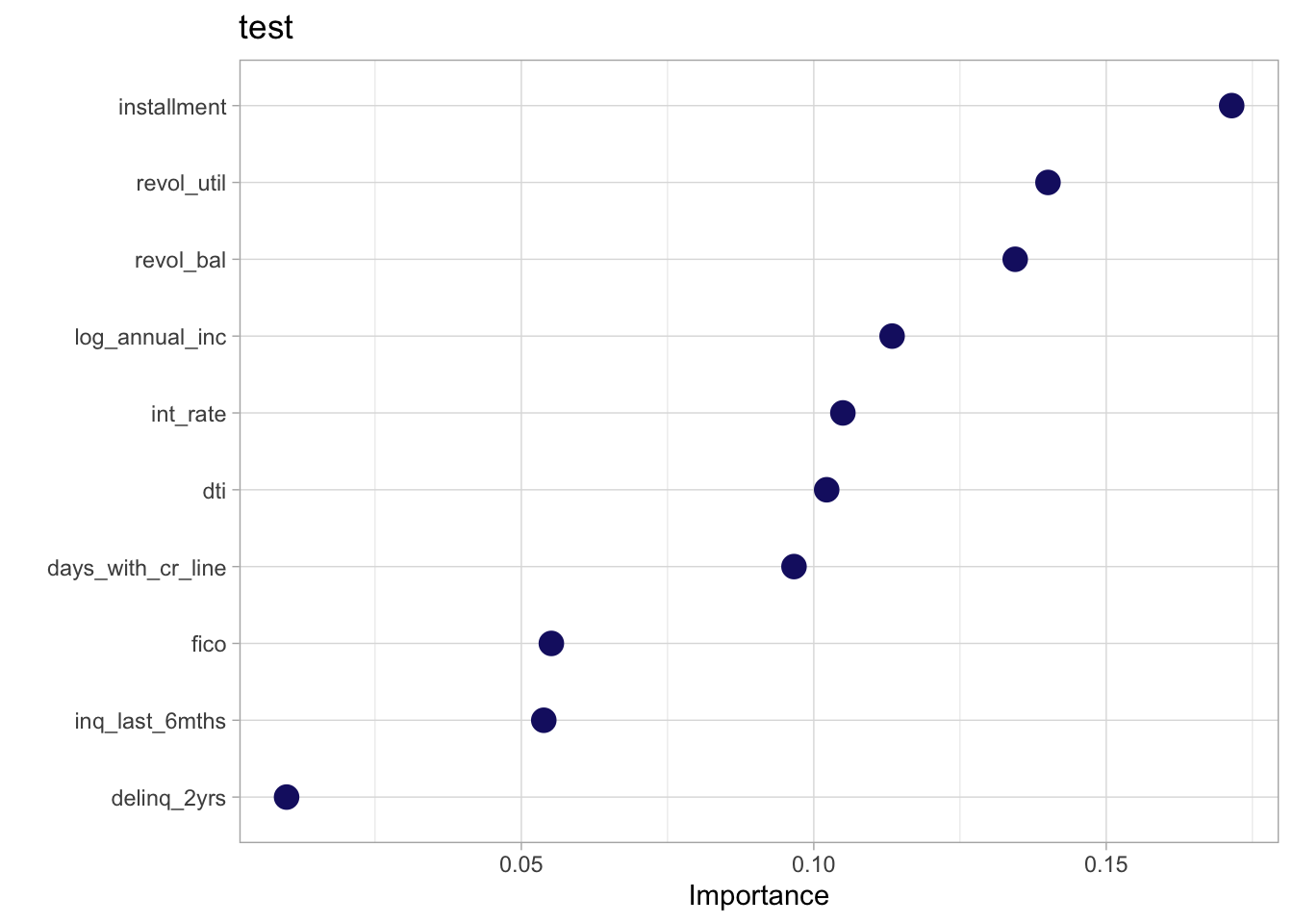
xgboost_workflow <-
  workflow() %>%
  add_recipe(xgboost_recipe) %>%
  add_model(xgboost_spec)

xgboost_grid <- grid_regular(
  parameters(xgboost_spec),
  levels = 3 )

set.seed(0826)
xgboost_tune <-
  tune_grid(xgboost_workflow,
            resamples = resamps,
            control = control_grid(),
            grid = xgboost_grid)

xgboost_tune %>%
  autoplot()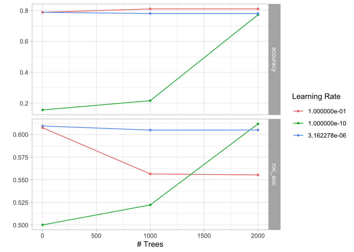
xg_best_params <- xgboost_tune %>%
  select_best(metric = 'accuracy')

xg_best_spec <- xgboost_spec %>%
  finalize_model(xg_best_params)

xg_final_fit <- workflow() %>%
  add_recipe(xgboost_recipe) %>%
  add_model(xg_best_spec) %>%
  last_fit(split = split)

xg_final_fit %>%
  collect_metrics() %>%
  gt() %>%
  tab_header(title = 'Payment status prediction results')  %>%
  tab_options(container.height = 400,
              container.overflow.y = TRUE,
              heading.background.color = "#21908CFF",
              table.width = "75%",
              column_labels.background.color = "black",
              table.font.color = "black") %>%
  tab_style(style = list(cell_fill(color = "#35B779FF")),
locations = cells_body())| Payment status prediction results | |||
|---|---|---|---|
| .metric | .estimator | .estimate | .config |
| accuracy | binary | 0.8258873 | Preprocessor1_Model1 |
| roc_auc | binary | 0.6187459 | Preprocessor1_Model1 |
Gabriel Mednick, PhD
Data scientist, biochemist, computational biologist, educator, life enthusiast