Palmer penguins
🐧 🐧 🐧 🐧 🐧 🐧 🐧 🐧 🐧 🐧 🐧 🐧 🐧 🐧 🐧 🐧 🐧 🐧 🐧 🐧 🐧 🐧 🐧 🐧 🐧 🐧 🐧
Introduction
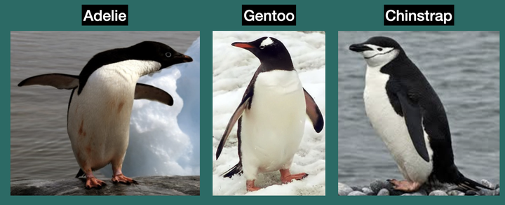
In this post, I use the Palmer penguins dataset from the palmerpenguins package to create a classification model for predicting penguin species. The data contains three penguin species and includes measurements of bill length, bill depth, flipper length and body mass. We will use bill length and depth as explanatory variables and accuracy will be the metric used to compare model performance. The following models are compared: multinomia lregression, random forest, k-nearest neighbors and xgboost.
After training these models and comparing the results, we will convert the R script into a command line tool that lets the user select a model and bill length and bill depth, and returns the predicted penguin species. If you find yourself predicting penguins in the Palmer Archipelago, this tool was made for you 😄!
library(tidyverse)
library(palmerpenguins) # maintained by Allison Horst
library(gt)
library(patchwork)
theme_set(theme_light())

#load data from the palmerpenguins package
palmer_df <- read_csv(path_to_file("penguins.csv"))

palmer_df %>% head() %>%
  gt() %>%
  tab_style(
    style = list(
      cell_fill(color = "#2D6A65"),
      cell_text(weight = "bold")
      ),
    locations = cells_body(
    )
)| species | island | bill_length_mm | bill_depth_mm | flipper_length_mm | body_mass_g | sex | year |
|---|---|---|---|---|---|---|---|
| Adelie | Torgersen | 39.1 | 18.7 | 181 | 3750 | male | 2007 |
| Adelie | Torgersen | 39.5 | 17.4 | 186 | 3800 | female | 2007 |
| Adelie | Torgersen | 40.3 | 18.0 | 195 | 3250 | female | 2007 |
| Adelie | Torgersen | NA | NA | NA | NA | NA | 2007 |
| Adelie | Torgersen | 36.7 | 19.3 | 193 | 3450 | female | 2007 |
| Adelie | Torgersen | 39.3 | 20.6 | 190 | 3650 | male | 2007 |
palmer_df %>%
  count(species) %>%
  gt() %>%
  tab_style(
    style = list(
      cell_fill(color = "#2D6A65"),
      cell_text(weight = "bold")
      ),
    locations = cells_body(
    )
)| species | n |
|---|---|
| Adelie | 152 |
| Chinstrap | 68 |
| Gentoo | 124 |
palmer_df %>%
  count(island) %>%
  gt() %>%
  tab_style(
    style = list(
      cell_fill(color = "#2D6A65"),
      cell_text(weight = "bold")
      ),
    locations = cells_body(
    )
)| island | n |
|---|---|
| Biscoe | 168 |
| Dream | 124 |
| Torgersen | 52 |
palmer_df %>%
  count(species, island) %>%
  gt() %>%
  tab_style(
    style = list(
      cell_fill(color = "#2D6A65"),
      cell_text(weight = "bold")
      ),
    locations = cells_body(
    )
) #since chinstrap and gentoo inhabit Dream and Biscoe repectively, it would not be a fair predictor variable| species | island | n |
|---|---|---|
| Adelie | Biscoe | 44 |
| Adelie | Dream | 56 |
| Adelie | Torgersen | 52 |
| Chinstrap | Dream | 68 |
| Gentoo | Biscoe | 124 |
palmer_df %>%
  summarize(min_year = min(year),
            max_year = max(year),
            observations = n(),
            missing_obs = sum(is.na(.))) %>%
  gt() %>%
  tab_style(style = list(cell_fill(color = "#2D6A65")), locations = cells_body()) %>%
  tab_style(
    style = list(
      cell_fill(color = "#2D6A65"),
      cell_text(weight = "bold")
      ),
    locations = cells_body(
    )
)| min_year | max_year | observations | missing_obs |
|---|---|---|---|
| 2007 | 2009 | 344 | 19 |
palmer_long <- palmer_df %>%
  drop_na() %>%
  pivot_longer(bill_length_mm:body_mass_g,
               names_to = "characteristic",
               values_to = "value")

palmer_long %>%
  group_by(species) %>%
 # filter(characteristic != "body_mass_g") %>%
  ggplot(aes(value, species, fill = species)) +
  geom_boxplot() +
  facet_wrap(~characteristic, scales = 'free_x') +
  theme(legend.position = 'none') +
  scale_fill_viridis_d()
palmer_long %>%
  group_by(species) %>%
 # filter(characteristic != "body_mass_g") %>%
  ggplot(aes(value, species, fill = sex)) +
  geom_boxplot() +
  facet_wrap(~characteristic, scales = 'free_x') +
  scale_fill_discrete(type = c("#DCE318FF", "#287D8EFF"))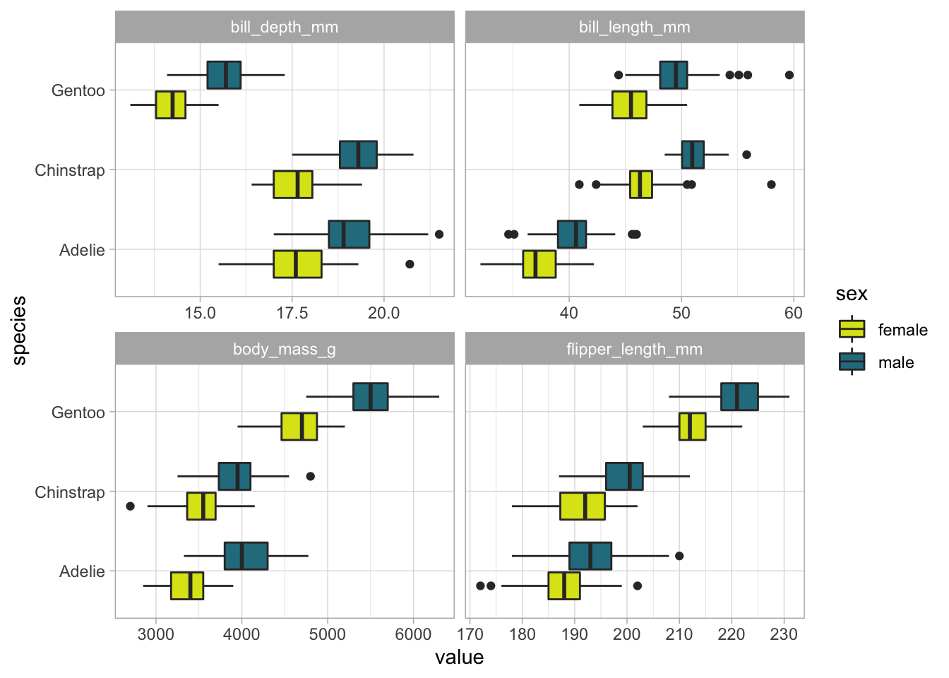
palmer_long %>%
  group_by(species) %>%
 # filter(characteristic != "body_mass_g") %>%
  ggplot(aes(value, fill = species)) +
  geom_density(alpha = 0.5) +
  facet_wrap(~characteristic, scales = 'free') +
  theme(legend.position = 'none') +
  scale_fill_viridis_d()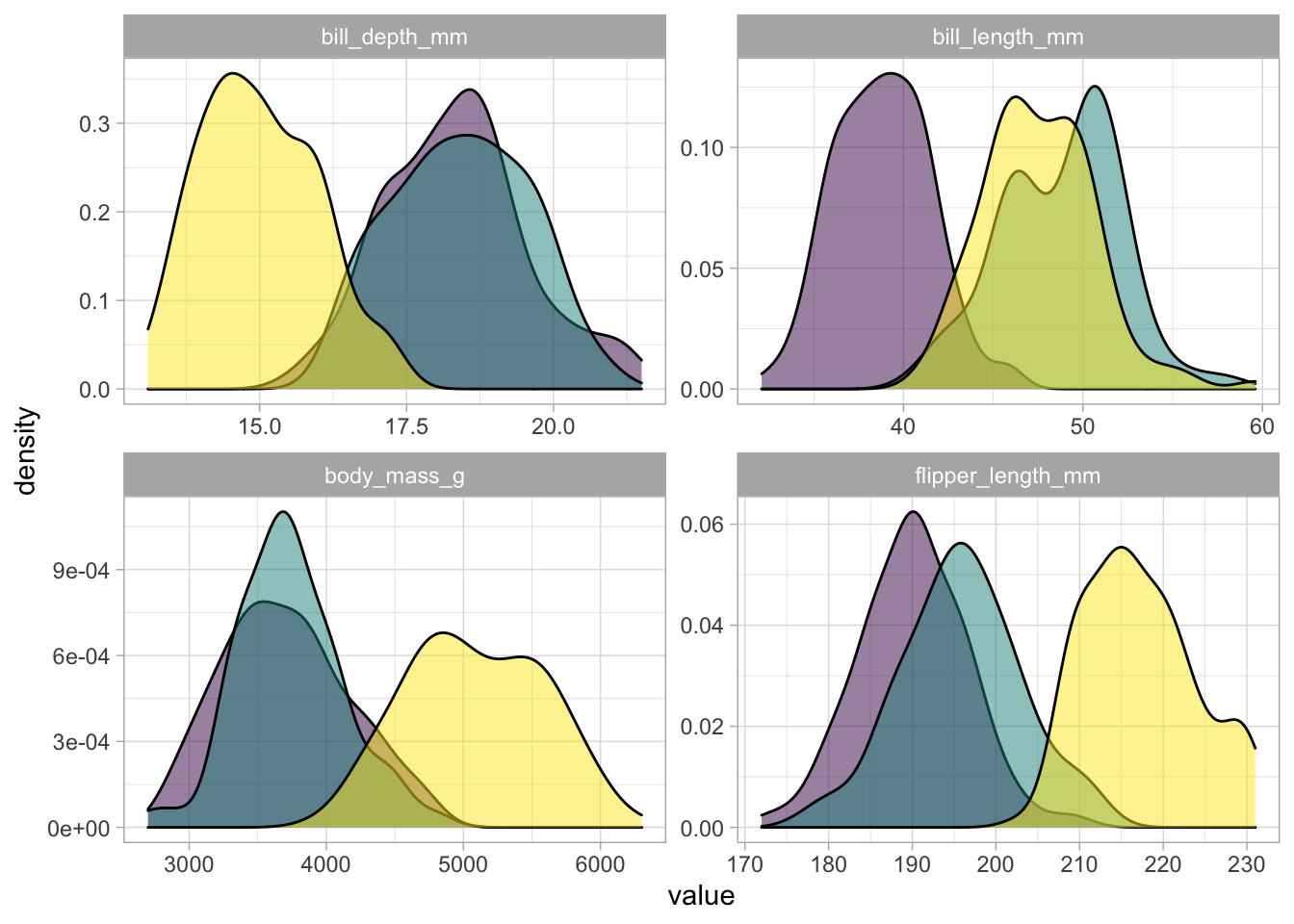
palmer_df %>%
  group_by(species) %>%
  drop_na() %>%
  summarize(`average bill depth` = median(bill_depth_mm),
            `average bill length` = median(bill_length_mm),
            `average body mass` = median(body_mass_g),
            `average flipper length` = median(flipper_length_mm)) %>%
  mutate(across(.cols = starts_with("average"), .fns = round))  %>% #across(.cols = everything(), .fns = NULL, ..., .names = NULL)
  gt() %>%
  tab_style(
    style = list(
      cell_fill(color = "#2D6A65"),
      cell_text(weight = "bold")
      ),
    locations = cells_body(
    )
)| species | average bill depth | average bill length | average body mass | average flipper length |
|---|---|---|---|---|
| Adelie | 18 | 39 | 3700 | 190 |
| Chinstrap | 18 | 50 | 3700 | 196 |
| Gentoo | 15 | 47 | 5050 | 216 |
Prediction model
library(tidymodels)
set.seed(777)

spl <- palmer_df %>% initial_split(prop = .8, strata = species)

palmer_train <- training(spl)

palmer_test <- testing(spl)

cv_resamples <- palmer_train %>% vfold_cv()
Before we can train our models, we need to decide which feature engineering steps are needed. We also need to specify the formula that tells our model what we are predicting and which explanatory features to use.
recipe_1 <- recipe(species ~ ., data = palmer_train) %>%
  step_impute_median(all_numeric_predictors()) %>%
  step_corr(all_numeric_predictors()) %>%
  step_impute_knn(sex) %>%
  step_dummy(all_nominal(), -all_outcomes()) %>%
  step_normalize(all_numeric_predictors())

recipe <- recipe(species ~ bill_length_mm + bill_depth_mm, data = palmer_train) %>%
  step_impute_median(all_predictors()) %>%
  step_normalize(all_predictors())
Create models, set modes and engines
mn_mod <- multinom_reg() %>%
  set_mode("classification") %>%
  set_engine('nnet')

rf_mod <- rand_forest() %>%
  set_mode("classification") %>%
  set_engine("ranger")

knn_mod <- nearest_neighbor() %>%
  set_mode("classification") %>%
  set_engine("kknn")

xg_mod <- boost_tree() %>%
  set_mode("classification") %>%
  set_engine("xgboost")
Weaving it together with workflow()
Multinomial regression model
mn_workflow <- workflow() %>%
  add_recipe(recipe) %>%
  add_model(mn_mod)

mn_mod_fit <- mn_workflow %>%
  fit(data = palmer_train)

mn_mod_preds <- mn_mod_fit %>%
  predict(new_data = palmer_test,
          type = 'class')

mn_results <- palmer_test %>%
  select(species) %>%
  bind_cols(mn_mod_preds)

metrics <- metric_set(accuracy, sens, spec)

metric_results <- mn_results %>%
  mutate_if(is.character, as.factor) %>%
  mutate(model = 'multinom_reg') %>%
  metrics(truth = species,
          estimate = .pred_class)

mn_p <- mn_results %>% conf_mat(.,
         truth = species,
         estimate = .pred_class) %>%
  autoplot(type = "heatmap") +
  ggtitle("Multinomial regression")
Random Forest model
rf_workflow <- workflow() %>%
  add_recipe(recipe) %>%
  add_model(rf_mod)

rf_mod_fit <- rf_workflow %>%
  fit(data = palmer_train)

rf_mod_preds <- rf_mod_fit %>%
  predict(new_data = palmer_test,
          type = 'class')

rf_results <- palmer_test %>%
  select(species) %>%
  bind_cols(rf_mod_preds)

rf_results %>%
  mutate_if(is.character, as.factor) %>%
  mutate(model = 'rf_mod') %>%
  metrics(truth = species,
          estimate = .pred_class)
## # A tibble: 3 × 3
## .metric .estimator .estimate
## <chr> <chr> <dbl>
## 1 accuracy multiclass 0.971
## 2 sens macro 0.976
## 3 spec macro 0.988rf_p <- rf_results %>% conf_mat(.,
truth = species,
estimate = .pred_class) %>%
autoplot(type = "heatmap") +
ggtitle("Random forest")K-nearest neighbors model
knn_workflow <- workflow() %>%
  add_recipe(recipe) %>%
  add_model(knn_mod)

knn_mod_fit <- knn_workflow %>%
  fit(data = palmer_train)

knn_mod_preds <- knn_mod_fit %>%
  predict(new_data = palmer_test,
          type = 'class')

knn_results <- palmer_test %>%
  select(species) %>%
  bind_cols(knn_mod_preds)

knn_results %>%
  mutate_if(is.character, as.factor) %>%
  mutate(model = 'knn_mod') %>%
  metrics(truth = species,
          estimate = .pred_class)
## # A tibble: 3 × 3
## .metric .estimator .estimate
## <chr> <chr> <dbl>
## 1 accuracy multiclass 0.971
## 2 sens macro 0.976
## 3 spec macro 0.986knn_p <- knn_results %>% conf_mat(.,
truth = species,
estimate = .pred_class) %>%
autoplot(type = "heatmap") +
ggtitle("k-nearest neighbors")Xgboost model
xg_workflow <- workflow() %>%
  add_recipe(recipe) %>%
  add_model(xg_mod)

xg_mod_fit <- xg_workflow %>%
  fit(data = palmer_train)
## [21:01:59] WARNING: amalgamation/../src/learner.cc:1095: Starting in XGBoost 1.3.0, the default evaluation metric used with the objective 'multi:softprob' was changed from 'merror' to 'mlogloss'. Explicitly set eval_metric if you'd like to restore the old behavior.xg_mod_preds <- xg_mod_fit %>%
predict(new_data = palmer_test,
type = 'class')
xg_results <- palmer_test %>%
select(species) %>%
bind_cols(xg_mod_preds)
metrics <- metric_set(accuracy, sens, spec)
xg_results %>%
mutate_if(is.character, as.factor) %>%
mutate(model = 'xgboost') %>%
metrics(truth = species,
estimate = .pred_class)## # A tibble: 3 × 3
## .metric .estimator .estimate
## <chr> <chr> <dbl>
## 1 accuracy multiclass 0.971
## 2 sens macro 0.976
## 3 spec macro 0.986xg_p <- xg_results %>% conf_mat(.,
truth = species,
estimate = .pred_class) %>%
autoplot(type = "heatmap") +
ggtitle("XGBoost")Confusion matrices
(mn_p + rf_p) / (knn_p + xg_p)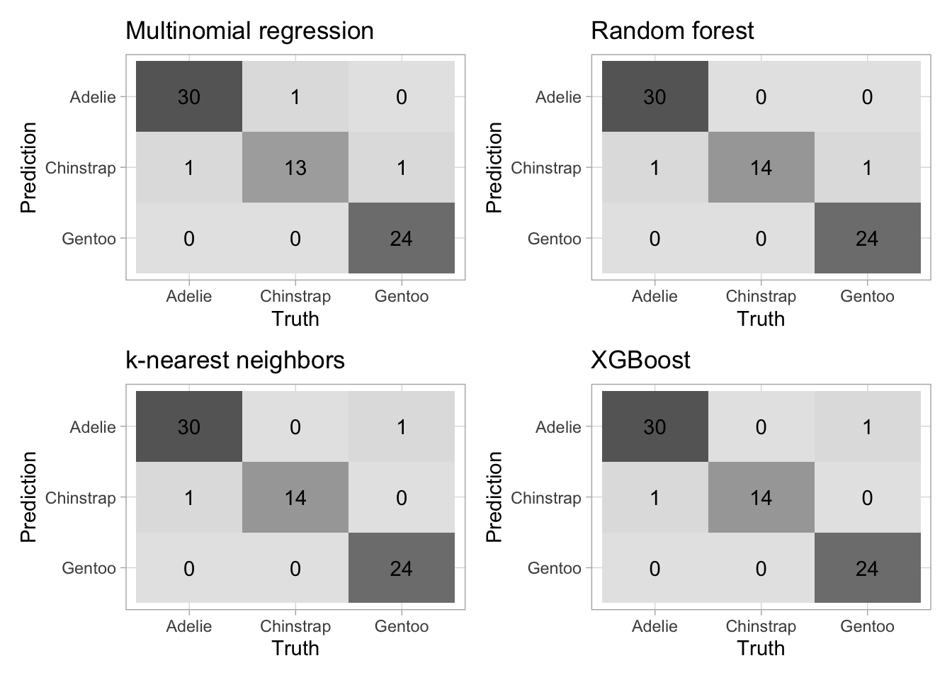
Results table
metric_results <- mn_results %>%
  mutate_if(is.character, as.factor) %>%
  mutate(model = 'multinom_reg') %>%
  metrics(truth = species,
          estimate = .pred_class) %>%
  bind_rows(rf_results %>%
  mutate_if(is.character, as.factor) %>%
  mutate(model = 'rf_mod') %>%
  metrics(truth = species,
          estimate = .pred_class)) %>%
  bind_rows(knn_results %>%
  mutate_if(is.character, as.factor) %>%
  mutate(model = 'knn_mod') %>%
  metrics(truth = species,
          estimate = .pred_class)) %>%
  bind_rows(xg_results %>%
  mutate_if(is.character, as.factor) %>%
  mutate(model = 'xg_mod') %>%
  metrics(truth = species,
          estimate = .pred_class)) %>%
  bind_cols(model_type = c('multinomial regression', 'multinomial regression', 'multinomial regression', 'random forest', 'random forest', 'random forest', 'knn', 'knn', 'knn', 'xgboost', 'xgboost', 'xgboost'))

metric_results %>%
  select(model = model_type, measure = `.metric`, value = `.estimate`) %>%
  filter(measure == 'accuracy') %>%
  arrange(-value) %>%
  gt() %>%
  tab_header(
    title = md("Summary of all four models"),
    subtitle = "Compaing model accuracies"
  ) %>%
  tab_style(
    style = list(
      cell_fill(color = "#2D6A65"),
      cell_text(weight = "bold")
      ),
    locations = cells_body(
    )
)| Summary of all four models | ||
|---|---|---|
| Compaing model accuracies | ||
| model | measure | value |
| random forest | accuracy | 0.9714286 |
| knn | accuracy | 0.9714286 |
| xgboost | accuracy | 0.9714286 |
| multinomial regression | accuracy | 0.9571429 |
penguin-prediction-tool
This tool uses classification algorithms to predict penguin species (Adelie, Chinstrap, Gentoo) based on bill length (mm) and bill depth (mm). Models include multinomial regression, k-nearest neighbors, random forest, xgboost (default hyperparameters settings were used).
The script utilizes the argparser package in R for parsing command-line arguments. The following examples show the incantation for running the Rscript in the command-line with the following arguments: model, bill length and bill depth.
Ex 1: Rscript penguin_sh_tool.R model=mn_mod_fit bill_length=39 bill_depth=18
Ex 2: Rscript penguin_sh_tool.R knn_mod_fit 50 18
Ex 3: Rscript penguin_sh_tool.R rf_mod_fit 50 18
Ex 4. Rscript penguin_sh_tool.R xg_mod_fit 50 14
In the command line, the output of Ex 3 includes the following messages

and returns the predicted species based on the user inputs.

If you want to make your own penguin predictions, the penguin prediction tool (R script) is available on GitHub
🐧 🐧 🐧 🐧 🐧 🐧 🐧 🐧 🐧 🐧 🐧 🐧 🐧 🐧 🐧 🐧 🐧 🐧 🐧 🐧 🐧 🐧 🐧 🐧 🐧 🐧 🐧
Gabriel Mednick, PhD
Data scientist, biochemist, computational biologist, educator, life enthusiast