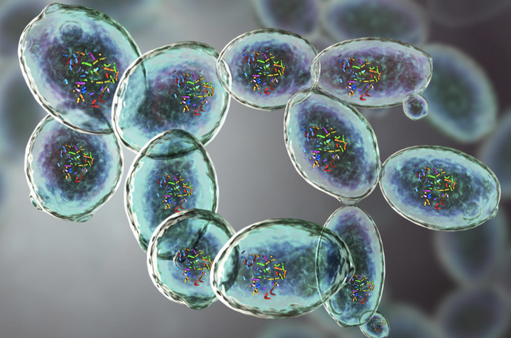
Exploring the yeast genome with Bioconductor
# load packages
library(tidyverse)
library(patchwork)
library(ggridges)
library(BSgenome)
library(glue)
library(GenomicRanges)
library(AnnotationHub)
library(org.Sc.sgd.db)
library(plyranges)
library(GenomicFeatures)
theme_set(theme_light())
library(Gviz)
library(ggbio)
library(BiocPkgTools)
library(biocViews)
What is Bioconductor
Bioconductor is a repository of packages for bioinformatics. Bioconductor contains over 5000 peer reviewed packages that can be categorized as data analysis software, experimental data or annotation data. We can explore the Bioconductor repository using the BiocPkgTools package.
Let’s visualize the package count by category and the most downloaded packages.
#library(BiocPkgTools)
pkgs <- biocDownloadStats()

pkgs %>%
  distinct(Package) %>%
  dplyr::count()
## # A tibble: 1 × 1
## n
## <int>
## 1 5646package_category <- pkgs %>% firstInBioc() %>%
group_by(repo) %>%
dplyr::count() %>%
ggplot(aes(n, fct_reorder(repo, n), fill = repo)) +
geom_col() +
labs(title = "Categories",
x = "Package count",
y = "",
color = "Category") +
theme(legend.position = 'none')
top_downloads <- pkgs %>%
group_by(Package) %>%
summarize(tot_downloads = sum(Nb_of_downloads)) %>%
slice_max(n = 30, tot_downloads) %>%
mutate(Package = fct_reorder(Package, tot_downloads)) %>%
ggplot(aes(tot_downloads, Package, fill = tot_downloads)) +
geom_col() +
theme(legend.position = "none") +
labs(title = "Top downloads",
x = "Total downloads",
y = "") +
scale_x_continuous(labels = scales::scientific) +
theme(axis.text.x = element_text(angle = 45, hjust = +1))
package_category | top_downloads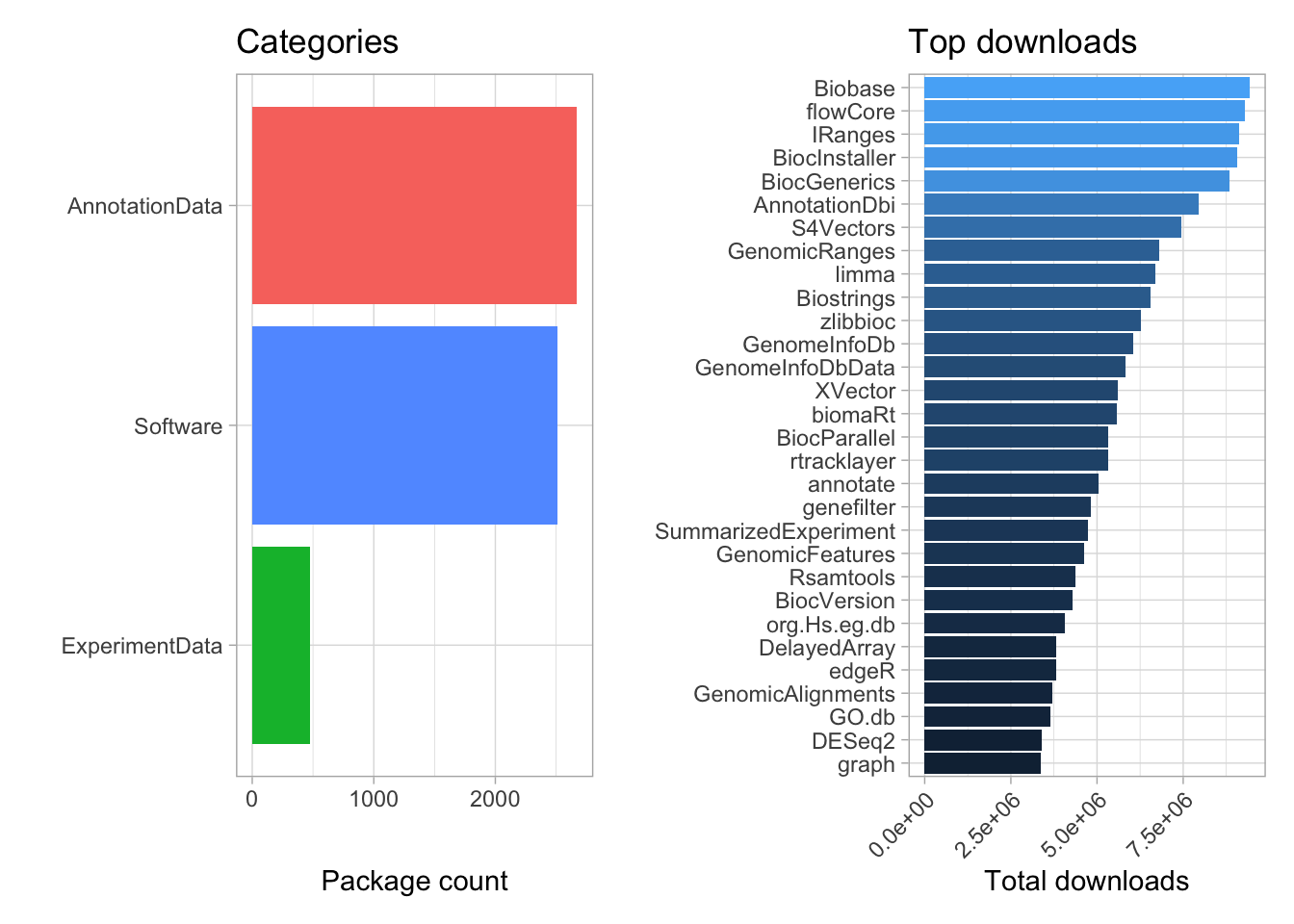
We can use the following incantation to visualize the most popular packages in each category.
library(tidytext)

pkgs %>%
  group_by(repo, Package) %>%
  summarize(tot_downloads = sum(Nb_of_downloads)) %>%
  ungroup() %>%
  group_by(repo) %>%
  slice_max(tot_downloads, n = 8) %>%
  mutate(repo = as.factor(repo),
         Package = reorder_within(Package, tot_downloads, repo)) %>%
  ggplot(aes(tot_downloads, Package, fill = repo)) +
  geom_col() +
  facet_wrap(~repo, scales = 'free', ncol = 1) +
  scale_y_reordered() +
  theme(legend.position = "none") +
  labs(title = "Most downloaded packages by category",
       x = "Total downloads",
       y = "") +
  theme(plot.title = element_text(hjust = 0))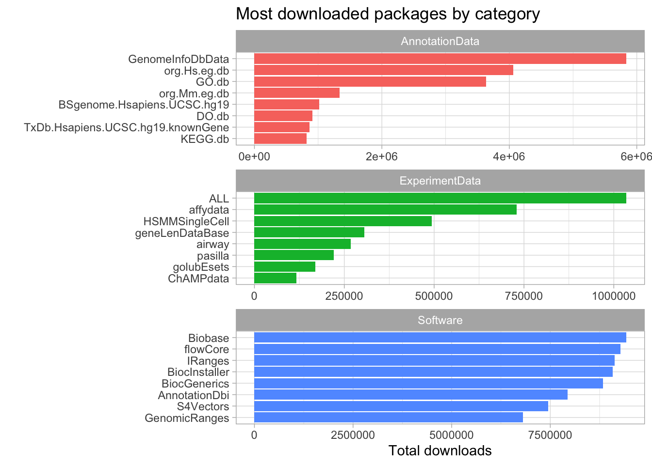
Let’s finish our exploration of the Bioconductor repository by looking at how the package count has grown over time in each category.
labels <- pkgs %>% group_by(repo) %>% summarize()
library(ggrepel)
pkgs %>%  firstInBioc() %>%
  group_by(Date, repo) %>%
  count() %>%
  ungroup() %>%
  group_by(repo) %>%
  mutate(tot_packages = cumsum(n),
         label = if_else(tot_packages == max(tot_packages), repo, NA_character_),
         label = glue("{repo} ({max(tot_packages)})")) %>%
  ggplot(aes(Date, tot_packages, color = label,)) +
  geom_line(size = 1) +
  labs(title = "Bioconductor package count over time",
       x = "Year",
       y = "Count",
color = "Category") 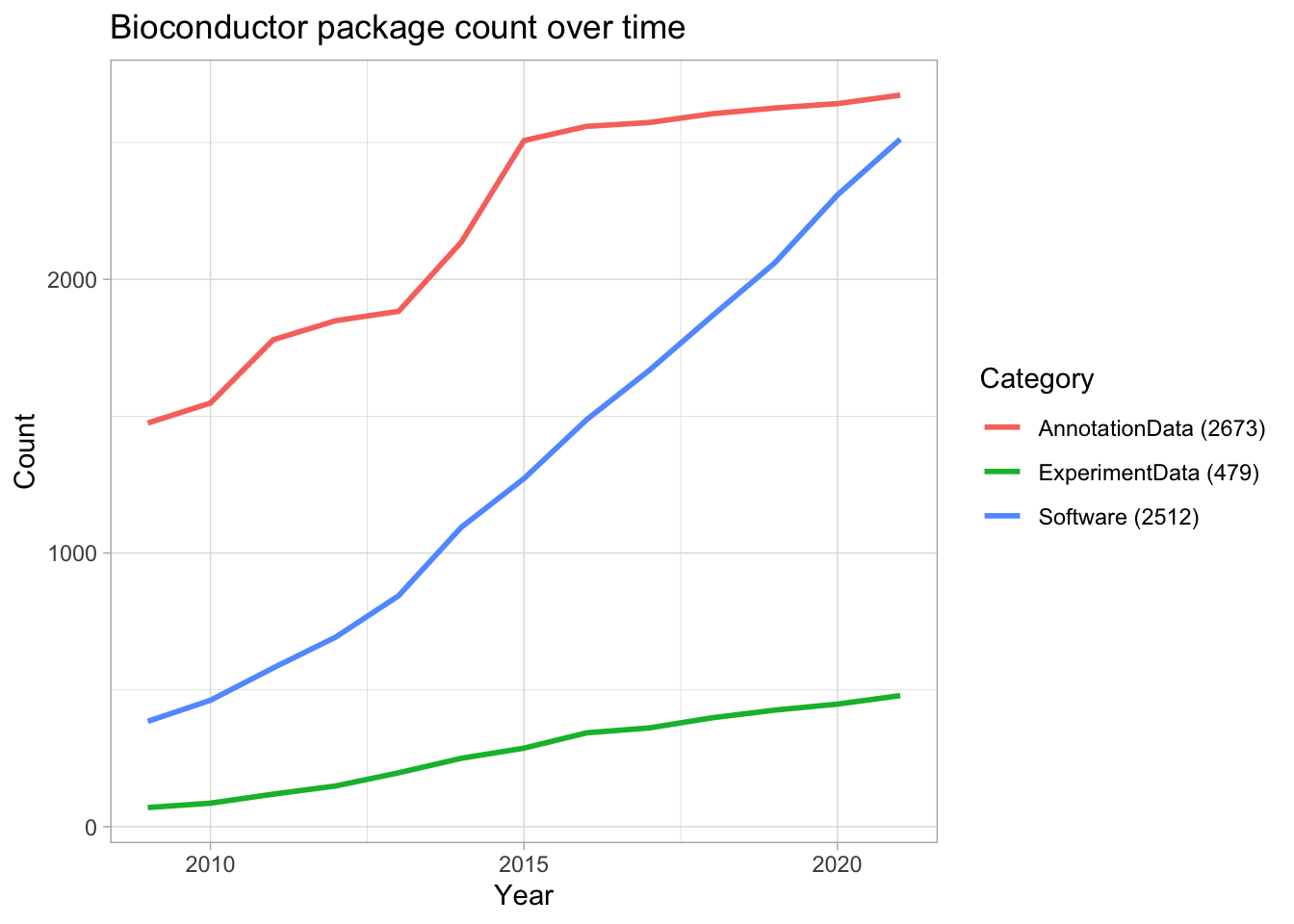
Diving into the yeast genome
To explore the yeast genome, we will use the BSgenome.Scerevisiae.UCSC.sacCer3 package to access yeast sequence data, TxDb.Scerevisiae.UCSC.sacCer3.sgdGene to access genetic ranges such as genes, transcripts, promoters, and use the org.Sc.sgd.db package to access various annotation sources.
These packages are available for other model organisms as well. For instance, we can load the BSgenome.Hsapiens.UCSC.hg19 package to access the human genome. The function, available.genomes(), provides a complete list of the available BSgenome objects.
# The complete list includes >100 genomes from UCSC
available.genomes() %>%
  head()
## [1] "BSgenome.Alyrata.JGI.v1"
## [2] "BSgenome.Amellifera.BeeBase.assembly4"
## [3] "BSgenome.Amellifera.NCBI.AmelHAv3.1"
## [4] "BSgenome.Amellifera.UCSC.apiMel2"
## [5] "BSgenome.Amellifera.UCSC.apiMel2.masked"
## [6] "BSgenome.Aofficinalis.NCBI.V1"Next let’s take a look inside the yeast BSgenome object.
library(BSgenome.Scerevisiae.UCSC.sacCer3)
library(Biostrings)

# Access the yeast genome
yeast <- BSgenome.Scerevisiae.UCSC.sacCer3
yeast
## Yeast genome:
## # organism: Saccharomyces cerevisiae (Yeast)
## # genome: sacCer3
## # provider: UCSC
## # release date: April 2011
## # 17 sequences:
## # chrI chrII chrIII chrIV chrV chrVI chrVII chrVIII chrIX
## # chrX chrXI chrXII chrXIII chrXIV chrXV chrXVI chrM
## # (use 'seqnames()' to see all the sequence names, use the '$' or '[[' operator
## # to access a given sequence)Use the following function to view a list of the available acessor functions for working with our BSgenome objects.
#The available BSgenome accessors are:
.S4methods(class = "BSgenome")
## [1] $ coerce show [[
## [5] autoplot length names as.list
## [9] seqinfo seqnames organism metadata
## [13] commonName countPWM export extractAt
## [17] getSeq injectSNPs masknames matchPWM
## [21] mseqnames provider providerVersion releaseDate
## [25] releaseName seqinfo<- seqnames<- snpcount
## [29] SNPlocs_pkgname snplocs sourceUrl vcountPattern
## [33] Views vmatchPattern vcountPDict vmatchPDict
## [37] bsgenomeName metadata<-
## see '?methods' for accessing help and source codeSequences derived from BSgenome objects are of the DNAString class and can be modified with functions from the Biostrings package.
class(yeast$chrI)## [1] "DNAString"
## attr(,"package")
## [1] "Biostrings"# provides a short description of the object
seqinfo(yeast)## Seqinfo object with 17 sequences (1 circular) from sacCer3 genome:
## seqnames seqlengths isCircular genome
## chrI 230218 FALSE sacCer3
## chrII 813184 FALSE sacCer3
## chrIII 316620 FALSE sacCer3
## chrIV 1531933 FALSE sacCer3
## chrV 576874 FALSE sacCer3
## ... ... ... ...
## chrXIII 924431 FALSE sacCer3
## chrXIV 784333 FALSE sacCer3
## chrXV 1091291 FALSE sacCer3
## chrXVI 948066 FALSE sacCer3
## chrM 85779 TRUE sacCer3# chromosome names
yeast %>%
seqnames()## [1] "chrI" "chrII" "chrIII" "chrIV" "chrV" "chrVI" "chrVII"
## [8] "chrVIII" "chrIX" "chrX" "chrXI" "chrXII" "chrXIII" "chrXIV"
## [15] "chrXV" "chrXVI" "chrM"The BSgenome object points to the genome object but does not import data into memory unless we ask for it. Let’s take a look at a couple of the functions for importing sequence data.
# Select chromosome sequence by name, one or many. And select start, end and or width:
getSeq(yeast, "chrM", end = 50)
## 50-letter DNAString object
## seq: TTCATAATTAATTTTTTATATATATATTATATTATAATATTAATTTATAT# alternative function to get specific sequence ranges
subseq(yeast$chrI, 1,100)## 100-letter DNAString object
## seq: CCACACCACACCCACACACCCACACACCACACCACA...CTAACACTACCCTAACACAGCCCTAATCTAACCCTGA custom summary function
For fun, let’s create a summary function that returns the name, length and GC percentage for each chromosome
# Yeast genome summary function: summarize_yeast_genome()
summarize_yeast_genome <- function() {

# Chromosome names and sequence lengths
#can also use org.Sc.sgdCHRLENGTHS from package: org.Sc.sgd.db
print("The length of each chromosome is as follows: ")
print(seqlengths(yeast))

#calculate GC percentage across chromosomes
print("We can use bsapply to calculate GC percent across all chromosomes: ")
param <- new("BSParams", X = Scerevisiae, FUN = letterFrequency)
#bsapply(param, "GC")
sum(unlist(bsapply(param, "GC")))/sum(seqlengths(yeast))
unlist(bsapply(param, "GC", as.prob = TRUE))

}

summarize_yeast_genome()
## [1] "The length of each chromosome is as follows: "
## chrI chrII chrIII chrIV chrV chrVI chrVII chrVIII chrIX chrX
## 230218 813184 316620 1531933 576874 270161 1090940 562643 439888 745751
## chrXI chrXII chrXIII chrXIV chrXV chrXVI chrM
## 666816 1078177 924431 784333 1091291 948066 85779
## [1] "We can use bsapply to calculate GC percent across all chromosomes: "## chrI.G|C chrII.G|C chrIII.G|C chrIV.G|C chrV.G|C chrVI.G|C
## 0.3927017 0.3834102 0.3853231 0.3790642 0.3850737 0.3872876
## chrVII.G|C chrVIII.G|C chrIX.G|C chrX.G|C chrXI.G|C chrXII.G|C
## 0.3806140 0.3849510 0.3890218 0.3837326 0.3806942 0.3847634
## chrXIII.G|C chrXIV.G|C chrXV.G|C chrXVI.G|C chrM.G|C
## 0.3820361 0.3863793 0.3816022 0.3806444 0.1710908Extracting the imp3 gene
After we introduce range objects and annotation, I will show how we can access a gene sequence by gene ID. Without that information, we need to know the ranges of the gene and create a custom GRanges object. Here, I use the Imp3 start and end sequence found here.
# imp3 yeast gene on chrVIII
imp3_start <- "ATGGTTAGAAAACTAAAGCATCATGAGCAAAAGTTATTGAAAAAAGTAGA"

imp3_end <- "CTAAGATCAAGAAAACCTTGTTGAGATACAGAAACCAAATCGACGATTTTGATTTTTCATAA"

# count occurrences of imp3_start to ensure there is only one match
countPattern(pattern=imp3_start,
                            subject=yeast[['chrVIII']],
                            max.mismatch = 2,
                            min.mismatch = 0)
## [1] 1The countPattern() function can be used to make sure that the sequence is found only once in the genome. The matchPattern() function, also from Biostrings, can be used to find the genomic coordinates.
# Calculate imp3_start and and imp3_end positions
imp3_start <- matchPattern(pattern=imp3_start,
             subject=yeast[['chrVIII']],
             max.mismatch = 2,
             min.mismatch = 0)

imp3_end <- matchPattern(pattern=imp3_end,
             subject=yeast[['chrVIII']],
             max.mismatch = 2,
             min.mismatch = 0)

# Create a GRanges object with coordinates of imp3
imp3_range <- GRanges(seqnames="chrVIII",
                        ranges=IRanges(start=393534,
                                       end=394085),
                        strand="+")
#GRanges("chrVIII", start = 393534, end = 394085)
After creating a GRanges object we can get the gene sequence with getSeq() and the amino acid sequence using translate().
# Extract imp3 sequence
Imp3_seq <- getSeq(yeast, names=imp3_range)
Imp3_seq
## DNAStringSet object of length 1:
## width seq
## [1] 552 ATGGTTAGAAAACTAAAGCATCATGAGCAAAAGT...AGAAACCAAATCGACGATTTTGATTTTTCATAAimp3_protein <- translate(Imp3_seq)
imp3_protein## AAStringSet object of length 1:
## width seq
## [1] 184 MVRKLKHHEQKLLKKVDFLEWKQDQGHRDTQVMR...RNMEDYVTWVDNSKIKKTLLRYRNQIDDFDFS*# A blast search confirms its sequence and length:
#https://www.ncbi.nlm.nih.gov/protein/AJU22745.1?report=genbank&log$=protalign&blast_rank=3&RID=NWXDKM0T01N
# alternative way to get imp3 using a BSgenome ranges and a txdb object (needs work)
# this will extract all gene sequences
# extractTranscriptSeqs(yeast,
# transcripts=yeast_genes)The complete sequence will not print to the console, so it is necessary to export the data to file to view the sequence. In order to do so, a fasta file can be generated with the function, writeXStringSet(yeastGeneSeqs,"yeastGeneSeqs.fa")
Working with TxDb objects
The TxDb package provides an efficient data container for extracting promoters, genes, exons and transcripts. There are TxDb packages for many model organisms but one can also create custom TxDb objects as well. The functions to work with TxDb objects are mostly from the GenomicFeatures package. When we use a function such as gene(), the function will return a GRanges object with the gene coordinates for each chromosome. The function .S4methods(class = 'GenomicRanges') provides a summary list of available methods to work with the GRanges object.
#BiocManager::install("TxDb.Scerevisiae.UCSC.sacCer3.sgdGene")
# .S4methods(class = 'GenomicRanges') find available methods
library(TxDb.Scerevisiae.UCSC.sacCer3.sgdGene)
#GenomicFeatures is loaded with the TxDb package

yeast_genome <- TxDb.Scerevisiae.UCSC.sacCer3.sgdGene
seqlevels(yeast_genome)
## [1] "chrI" "chrII" "chrIII" "chrIV" "chrV" "chrVI" "chrVII"
## [8] "chrVIII" "chrIX" "chrX" "chrXI" "chrXII" "chrXIII" "chrXIV"
## [15] "chrXV" "chrXVI" "chrM"yeast_genes <- genes(yeast_genome)
# ggbio
autoplot(yeast_genes, layout = 'karyogram', color = 'lightblue', coverage.col = "gray50") +
labs(title = "Karyogram layout displaying gene distribution") 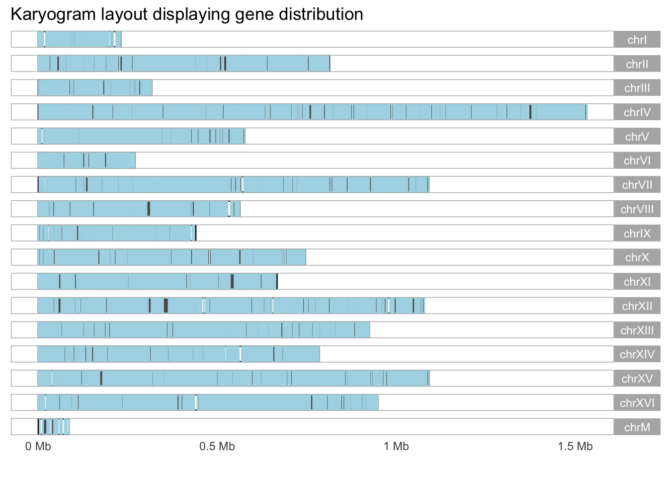
# Let's extract all transcript sequences
yeastGeneSeqs <- getSeq(yeast, names=yeast_genes)
yeastGeneSeqs
## DNAStringSet object of length 6534:
## width seq names
## [1] 464 ATATATTATATTATATTTTTAT...AATATACTTTATATTTTATAA Q0010
## [2] 291 ATATTAATAATATATATATTAT...AAGTTTTTATATTCATTATAA Q0032
## [3] 12884 ATGGTACAAAGATGATTATATT...ACACCAGCTGTACAATCTTAA Q0055
## [4] 1100 ATATTAATATTATTAATAATAA...CATTATAACAATATCGAATAA Q0075
## [5] 147 ATGCCACAATTAGTTCCATTTT...TTATTTATTTCTAAATTATAA Q0080
## ... ... ...
## [6530] 393 ATGGTAAGTTTCATAACGTCTA...AAATTGATTGTTAGTGGTTGA YPR200C
## [6531] 1215 ATGTCAGAAGATCAAAAAAGTG...ATATGGAACAATAGAAATTAA YPR201W
## [6532] 1157 ATGGAAATTGAAAACGAACGTA...CATGTGTGCTGCCCAAGTTGA YPR202W
## [6533] 483 ATGATGCCTGCTAAACTGCAGC...CAGCATTCTCTCCACAGCTAG YPR204C-A
## [6534] 3099 ATGGCAGACACACCCTCTGTGG...AGCAGAGAAGTTGGAGAGTGA YPR204WIncorporating ggplot2
In order to use ggplot2, we need to extract a GRanges object from the TxDb object and then convert it into a tibble.
yeast_genes_df <- yeast_genes %>%
  as_tibble()

tot_yeast_genes <- yeast_genes_df %>%
  summarize(n=n())

# plotting gene count by chromosome
yeast_genes_df %>%
  group_by(seqnames) %>%
  add_count(seqnames) %>%
  mutate(chromosome_gene = glue("{seqnames} ({n} genes)")) %>%
  group_by(chromosome_gene) %>%
  ggplot(aes(n, fct_reorder(chromosome_gene, n), fill = n)) +
  geom_col() +
  theme(legend.position = 'none') +
  labs(title = expression(paste("Gene count by chromosome for ", italic("S. cerevisiae"))),
       subtitle = "Total genes = 6534",
       x = 'Gene count',
       y = "")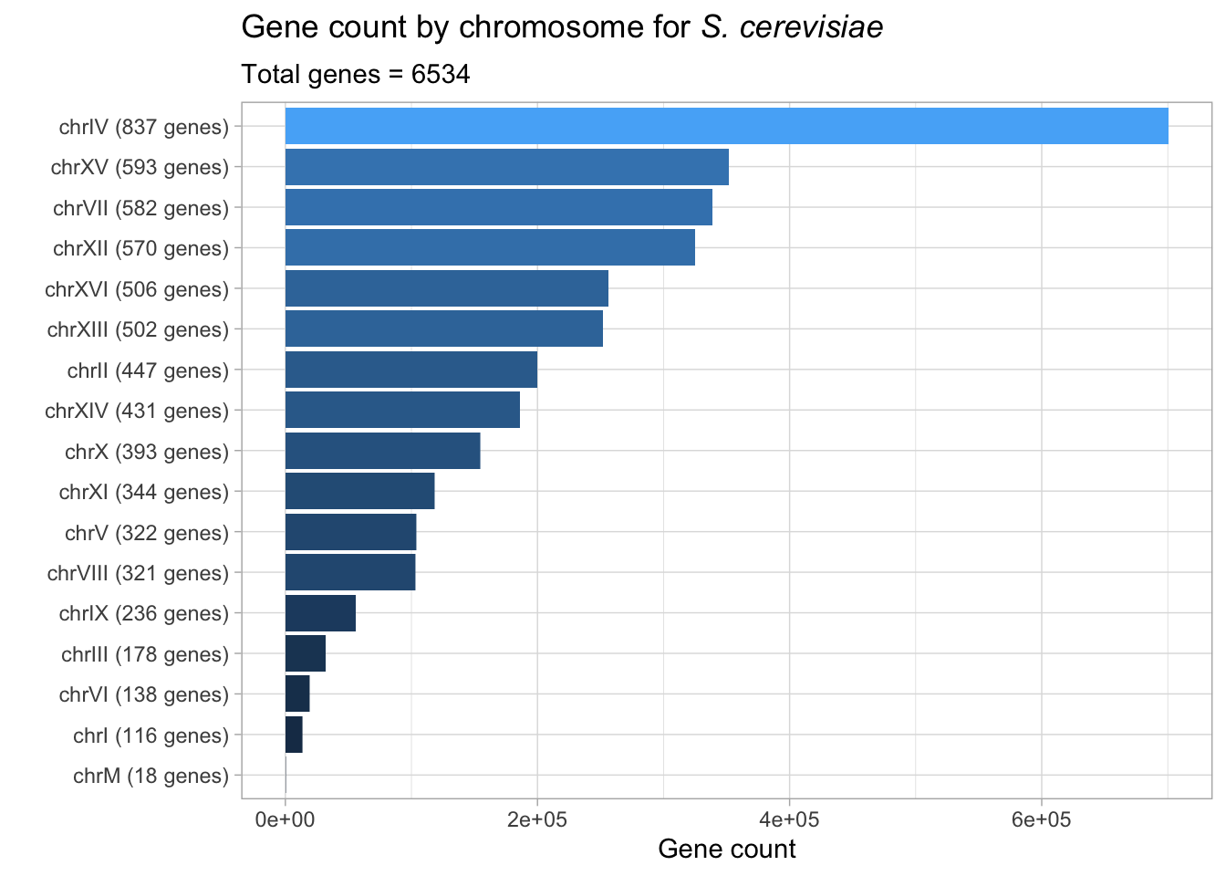
Since we also have data on gene widths, we can plot the count density of gene width. The aesthetic, geom_density_ridges() from the GGridges package provides a nice way to visualize gene width across chromosomes.
# I prefer the geom_density_ridges for viewing gene widths across chromosomes
# yeast_genes_df %>%
#   group_by(seqnames) %>%
#   mutate(avg_width = mean(width)) %>%
#   add_count(seqnames) %>%
#   ggplot(aes(width, fill = avg_width)) +
#   geom_density() +
#   facet_wrap(~seqnames, scales = "free_y") +
#   scale_fill_viridis_c(alpha = 0.8) +
#   labs(title = 'Distribution of gene width for each chromsome',
#       x="Gene width density (log)",
#       y = "",
#       fill = "Avg width") +
#   scale_x_log10()


yeast_genes_df %>%
  group_by(seqnames) %>%
  mutate(avg_width = mean(width)) %>%
  add_count(seqnames) %>%
  ggplot(aes(width, seqnames, fill = avg_width), group = seqnames) +
  geom_density_ridges() +
  scale_fill_viridis_c(alpha = 0.8) +
  labs(title = 'Density distribution of gene length by chromsome',
      x="Gene length",
      y = "") +
  theme(legend.position = "none")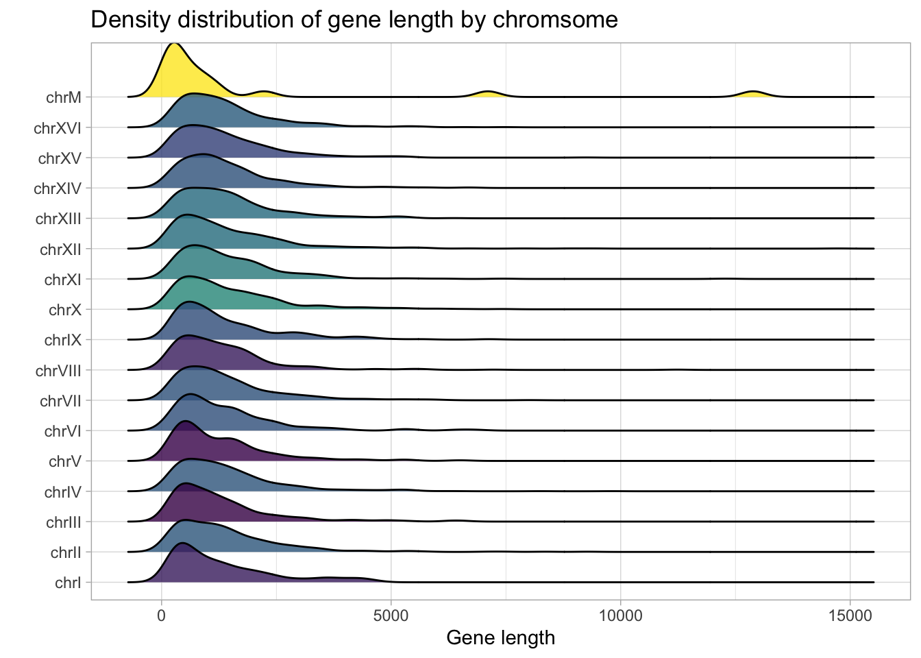
Annotation
We can annotate our GRanges object using the org.Sc.sgd.db package which includes various annotation sources such as GEO and ENCODE. Here, I’m going to add the common name and description for each gene. We will then use the tidytext package to explore the most common words associated with each chromosome.
#columns(org.Sc.sgd.db::org.Sc.sgd.db) to look at annotation options
# that can be provided to the column argument
yeast_genes_df <- yeast_genes_df %>%
  mutate(common_name = AnnotationDbi::mapIds(org.Sc.sgd.db::org.Sc.sgd.db,
                                        keys = gene_id,
                                        keytype = "ENSEMBL",
                                        column = "COMMON",
                                        multiVals = "first")) %>%
  mutate(description = AnnotationDbi::mapIds(org.Sc.sgd.db::org.Sc.sgd.db,
                                        keys = gene_id,
                                        keytype = "ENSEMBL",
                                        column = "DESCRIPTION",
                                        multiVals = "first"))

yeast_genes_df %>% filter(common_name == "IMP3")
## # A tibble: 1 × 8
## seqnames start end width strand gene_id common_name description
## <fct> <int> <int> <int> <fct> <chr> <chr> <chr>
## 1 chrVIII 393534 394085 552 + YHR148W IMP3 Component of the SSU …Let’s use this information to isolate genes that include the word ‘kinase’ in their descriptions.
#Let's use the description annotation to sort kinases and display them using the karyogram layout
kinase_karyogram <- yeast_genes_df %>%
  drop_na() %>%
  filter(grepl("kinase", description)) %>%
  as_granges()

kinase_karyogram %>%
  autoplot(layout = "karyogram", color = 'darkblue') +
  labs(title = "Distribution of kinases in the yeast genome")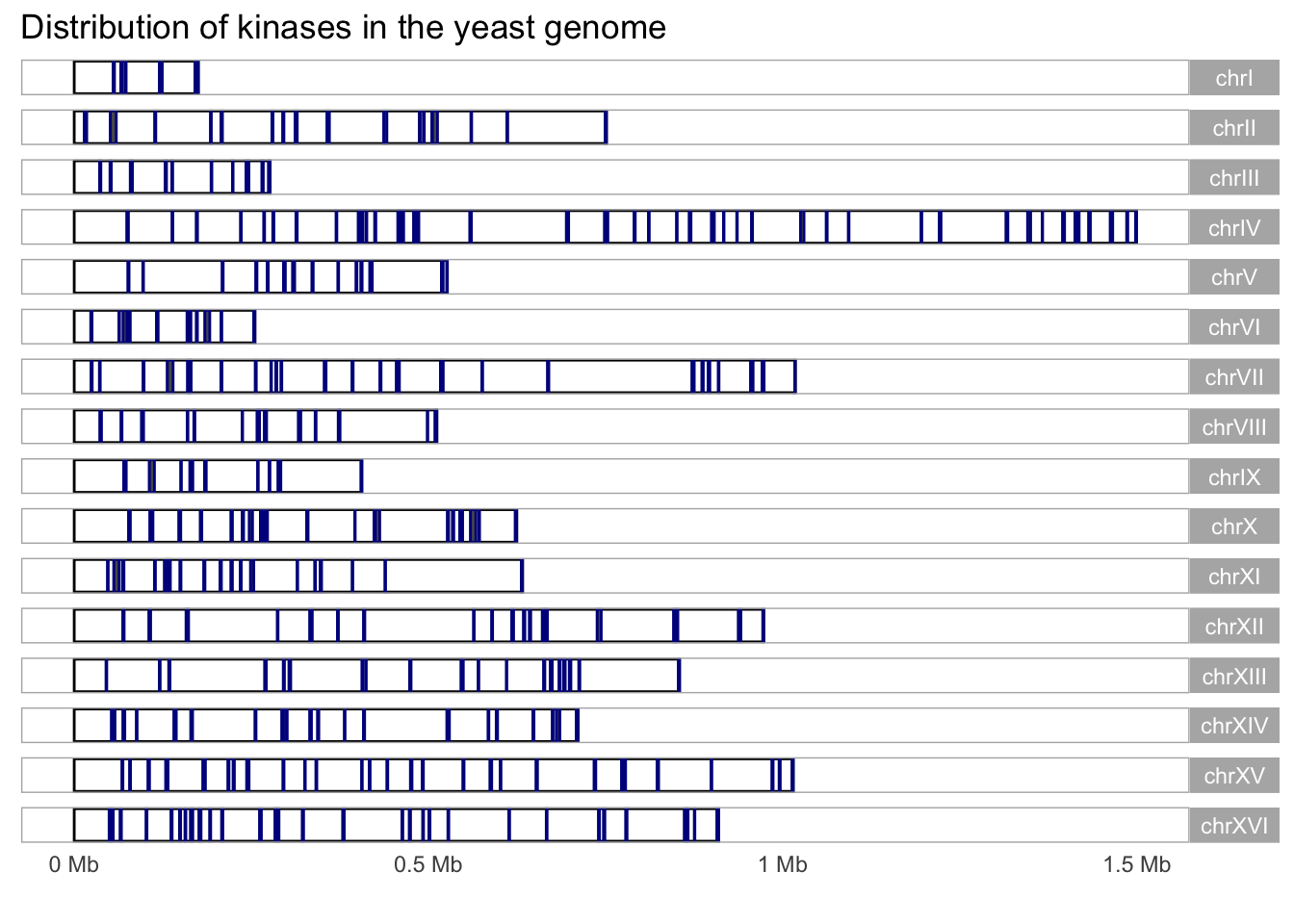
We can also use the gene descriptions to find the most frequent words associated with each chromosome. We will use the Tidytext package to facilitate this analysis.
library(tidytext)
yeast_genes_df %>%
  drop_na() %>%
  unnest_tokens('word', 'description') %>%
  anti_join(stop_words, by = 'word') %>%
  count(seqnames, word, sort=T) %>%
  group_by(seqnames) %>%
  slice_max(n, n=5) %>%
  ungroup() %>%
  mutate(word = reorder_within(word, n, seqnames)) %>%
  ggplot(aes(n, word, fill = seqnames)) +
  geom_col() +
  facet_wrap(~seqnames, scales = "free") +
  scale_y_reordered() +
  labs(
    x = "Word frequency", y = NULL,
    title = "Top words from gene description annotation by chromosome"
  ) +
  theme(legend.position = "none") +
  theme(axis.title.x=element_blank(),
        axis.text.x=element_blank(),
        axis.ticks.x=element_blank())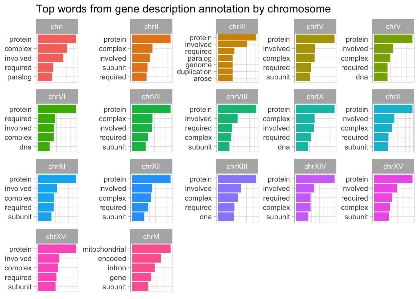
A more interesting selection of words can be found by selecting the unique words associated with each chromosome. We can do this by using the TF-IDF algorithm.
common_words <- c("protein","involved", "required", "complex", "subunit", "involved", "dna")
tfidf <- yeast_genes_df %>%
  drop_na() %>%
  unnest_tokens('word', 'description') %>%
  filter(!word %in% common_words) %>%
  anti_join(stop_words, by = 'word') %>%
  dplyr::count(seqnames, word, sort=T) %>%
  group_by(seqnames) %>%
  slice_max(n, n=5)

tfidf %>%
  bind_tf_idf(word, seqnames, n) %>%
  group_by(seqnames) %>%
  #slice_max(tf_idf, n=12) %>%
  ungroup() %>%
  mutate(word = reorder_within(word, tf_idf, seqnames)) %>%
  ggplot(aes(tf_idf, word, fill = seqnames)) +
  geom_col() +
  facet_wrap(~seqnames, scales = "free") +
  scale_y_reordered() +
  labs(
    x = "Word frequency", y = NULL,
    title = "TF_IDF algorithm"
  ) +
  theme(legend.position = "none") +
  labs(x = "",
       y = "TF-IDF of chromosome-word pairs") +
  theme(axis.title.x=element_blank(),
        axis.text.x=element_blank(),
        axis.ticks.x=element_blank())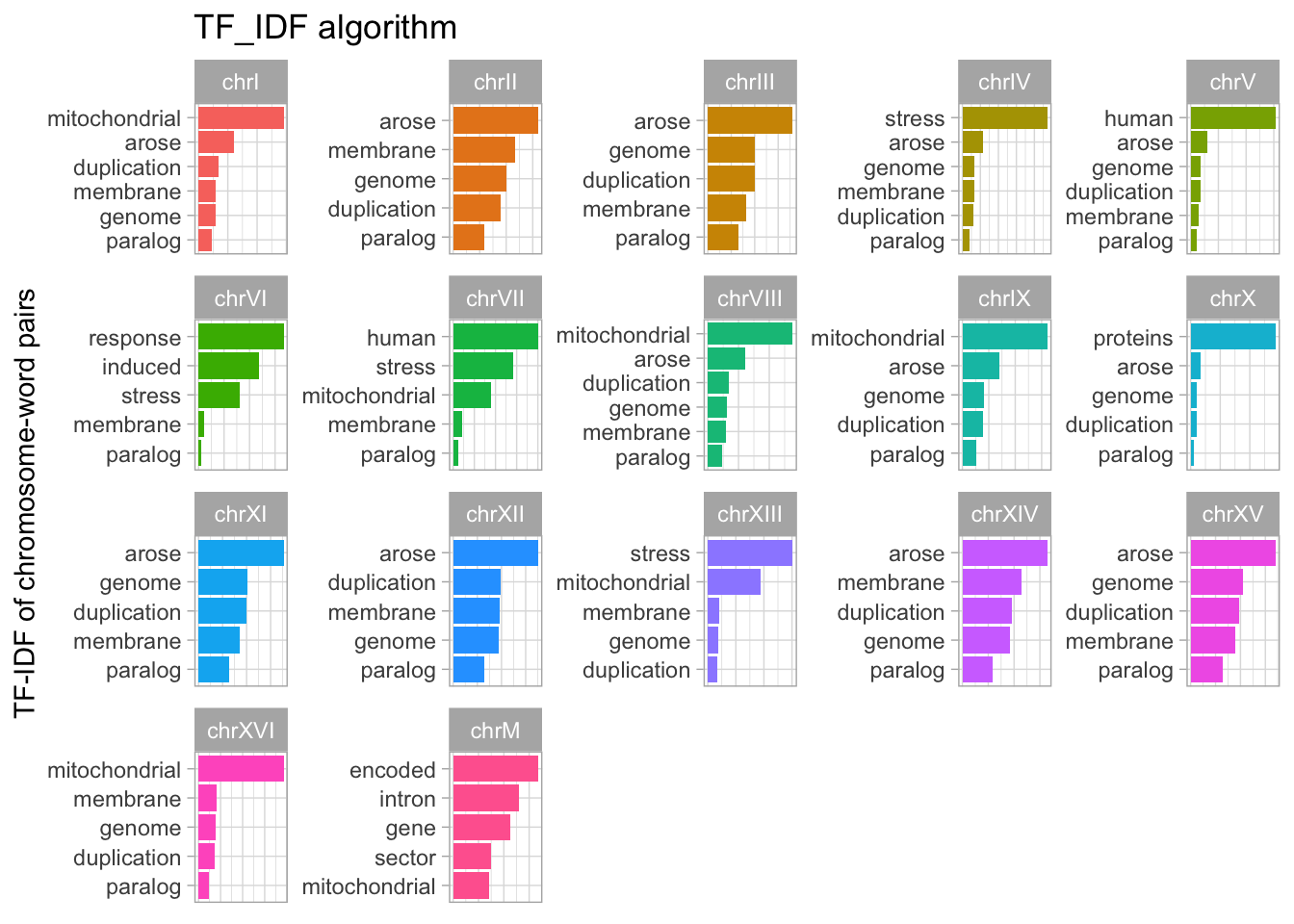
Summary
This post introduced several core Bioconductor packages for accessing, annotating and manipulating genomic data. We used packages such as Biostrings, GenomicRanges, GenomicFeatures, Plyranges and ggbio. Finally, we utilized the tidy data framework and used packages such as Dplyr, GGplot2 and the Tidytext package for natural language processing. In a follow up post, I plan to dive deeper into the yeast genome using data from the yeastExpData and yeastNagalakshmi packages.
Gabriel Mednick, PhD
Data scientist, biochemist, computational biologist, educator, life enthusiast